![]()
Programming for Data Analysis Assignment 2019
Explain the use of the numpy.random package in Python including detailed explanations of at least five of the distributions provided for in the package.
There are four distinct task to be carried out in this Jupyter Notebook.
- Explain the overall purpose of the package.
- Explain the use of the “Simple random data” and “Permutations” functions.
- Explain the use and purpose of at least five “Distributions” functions.
- Explain the use of seeds in generating pseudorandom numbers.
Table of contents
- Python libraries used for this assignment
- Task 1: Explain the overall purpose of the package
- Task 2: Explain the use of the Simple random data and Permutations functions.
- Task 3: Explain the use and purpose of at least five “Distributions” functions
- Task 4: Explain the use of seeds in generating pseudorandom numbers
Python libraries used
To run this notebook the following some python libraries must be imported. This notebook uses the numpy, pandas, seaborn and matplotlib python libraries which are installed with the Anaconda distribution.
As the examples in this asignment generate arrays of floating point numbers, I have set the print options for ease of reading using numpy.set_printoptions. This determines the way floating point numbers, arrays and other NumPy objects are displayed.
Jupyter notebook will usually only print the output of the last statement. However this can be changed using the InteractiveShell settings. I did use this at the start but it makes the document too long.
# import libraries using common alias names
import numpy as np
import pandas as pd
import seaborn as sns
import matplotlib.pyplot as plt

#np.version.version  # check what version of packages are installed.
print("NumPy version",np.__version__, "pandas version ",pd.__version__, "seaborn version",sns.__version__  )  # '1.16.2'

#np.set_printoptions(formatter={'float': lambda x: "{0:6.3f}".format(x)})
np.set_printoptions(precision=4)  # set floating point precision to 4
np.set_printoptions(threshold=5) # summarise long arrays
np.set_printoptions(suppress=True) # to suppress small results

#from IPython.core.interactiveshell import InteractiveShell
#InteractiveShell.ast_node_interactivity = "all"  #
import warnings
warnings.filterwarnings('ignore')
Task 1. Explain the overall purpose of the package numpy.random
NumPy, short for Numerical Python, is one of the most important foundational packages for numerical and scientific computing in Python and many other Python packages that are used for data analytics and machine learning are built on NumPy such as pandas, scikit-learn among others. NumPy provides a multidimensional array object, various derived objects (such as masked arrays and matrices), and an assortment of routines for fast operations on arrays, including mathematical, logical, shape manipulation, sorting, selecting, I/O, discrete Fourier transforms, basic linear algebra, basic) statistical operations, random simulation and much more. (w3 numpy tutorial
numpy.random is a sub-package of NumPy for working with random numbers and is somewhat similar to the Python standard library random but works with NumPy's arrays. It can create arrays of random numbers from various statisitical probability distributions and also randomly sample from arrays or lists. NumPy's random module is frequently used to fake or simulate data which is an important tool in data analysis, scientific research, machine learning and other areas. The simulated data can be analysed and used to test methods before applying to the real data.
A NumPy ndarray can be created using the NumPy array function which takes any sequence-like objects such as lists, nested lists etc. Other NumPy functions can create new arrays including zeros, ones, empty, arange, full and eye among others as detailed in the numpy quickstart tutorial. NumPy's random module also creates ndarray objects.
Some key points about any of NumPy's ndarray objects which are relevant to the numpy.random module:
- The data in an ndarray must be homogeneous, that is all of it's data elements must of the same type.
- Arrays have a ndim attribute for the number of axes or dimensions of the array
- Arrays have a shape attribute which is a tuple that indicates the size of the array in each dimension. The length of the shape tupple is the number of axes that the array has.
- Arrays have a dtype attribute which is an object that describes the data type of the array.
- The
sizeattribute is the total number of elements in the array.
Python's standard library random already provides a number of tools for working with random numbers. However it only samples one value at a time while numpy.random can efficiently generate arrays of sample values from various probability distributions and also provides many more probability distributions to use. NumPy's random module is generally much much faster and more efficient than the stdlib random particularly when working with lots of samples, however the random module may be sufficient and more efficient for other simpler purposes.
As well as being able to generate random sequnces, NumPy's random also has functions for randomly sampling elements from an array or sequence of elements, numbers or otherwise.
Both of these random modules generate pseudorandom numbers rather than actual random numbers. Computer programs are deterministic because their operation is predictable and repeatable. They produce outputs based on inputs and according to a set of predetermined steps or rules so therefore it is not really possible for a computer to generate truly random numbers. These random modules implements pseudorandom numbers for various distributions that may appear random they are not truly so.
According to wolfram mathworld a random number
is a number chosen as if by chance from some specified distribution such that selection of a large set of these numbers reproduces the underlying distribution. Almost always, such numbers are also required to be independent, so that there are no correlations between successive numbers. Computer-generated random numbers are sometimes called pseudorandom numbers, while the term "random" is reserved for the output of unpredictable physical processes. When used without qualification, the word "random" usually means "random with a uniform distribution." Other distributions are of course possible.
There are many computational and statistical methods that use random numbers and random sampling. Gaming and gambling applications involve randomness. Scientific and numerical disciplines use it for hypothesis testing. Statistics and probability involve the concept of randomness and uncertainty. Monte carlo simulation uses random numbers to simulate real world problems. Monte Carlo methods, or Monte Carlo experiments, are a broad class of computational algorithms that rely on repeated random sampling to obtain numerical results. The underlying concept is to use randomness to solve problems that might be deterministic in principle. Monte-carlo simulators are often used to assess the risk of a given trading strategy say with options or stocks. A monte carlo simulator can help one visualize most or all of the potential outcomes to have a much better idea regarding the risk of a decision.
Being able to randomly generate or select elements from a set has many uses in software applications such as gaming. Randomness has many uses in science, art, statistics, cryptography, gaming, gambling, and other fields. For example, random assignment in randomized controlled trials helps scientists to test hypotheses, and random numbers or pseudorandom numbers help video games such as video poker*. Applications of randomness.
The ability to generate sets of numbers with properties from a particular probability distribution is also very useful for simulating a dataset, maybe prior to the real dataset becoming available but also for demonstrating of and learning statistical and data analysis concepts.
Data Analytics and Machine learning projects frequently use random sampling on actual datasets for testing and evaluation analytical methods and algorithms. A set of samples of data are studied and then use to try and predict the properties of unknown data. In machine learning, a dataset can be split into training and test set where the dataset is shuffled and a classifier is built with a randomly selected subset of the dataset and the classifier is then tested on the remaining subset of the data. A train-test split is used for model selection and cross validation purposes.
According to scikit-learn.
Machine learning is about learning some properties of a data set and then testing those properties against another data set. A common practice in machine learning is to evaluate an algorithm by splitting a data set into two. We call one of those sets the training set, on which we learn some properties; we call the other set the testing set, on which we test the learned properties.
The machine learning algorithms in the scikit-learn package use numpy.random in the background. There is a random element to the train_test split as it uses numpy random to randomly choose elements for the training array and the test array. Cross validation methods such as k-fold validation randomly sploit the original dataset into training and testing subset many times.
Task 2. Explain the use of the “Simple random data” and “Permutations” functions.
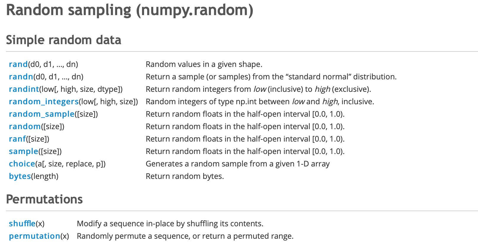
The Numpy random module contains some simple random datafunctions for random sampling of both discrete and continuous data from the uniform, normal or standard normal probability distributions and for randomly sampling from a sequence or set of elements. It also has two permutations function for shuffling arrays. These functions all return either arrays of random values where the number of dimensions and the number of elements can be specified or scalar values. For this assignment, I have separated the ten simple random data functions into groups according to the type of distribution they draw from and the type of number returned. Some of these functions appear to do the same thing and some are variants of the distribution functions for the Uniform and Normal distributions which are covered in more detail in Task 3 below.
Simple random data functions
- Random samples from the Normal and Standard Normal Distributions (floats)
- Random samples from the Continuous Standard Uniform Distribution (floats)
- Random samples from the Continuous Uniform Distribution (floats)
- Random samples from the Discrete Uniform Distribution (integers)
- Random samples from a given array of elements
- Random bytes
Permutations functions
Random samples from the Standard Normal Distributions (floats)
The numpy.random randn() function returns a sample (or samples) of random values from the standard normal distribution, also known as the univariate normal Gaussian distribution, that has a mean of 0 and variance of 1. This
The size of the sample returned and the shape of the can be specified or else a single float randomly sampled from the distribution is returned. You can also get random samples from other Normal distributions with a specified mean and variance $N(\mu, \sigma^2)$ by scaling the values by multiplying the output of the rand function by $\sigma$ and adding $\mu$ where the standard deviation $\sigma$ is the square root of the variance $\sigma^2$.
numpy.random.randn() is a convenience function for the numpy.random.standard_normal function which takes a tuple for the size and shape dimensions and is covered in more detail in Task 3.
Using numpy.random.randn function.
rand can be used to create various sized arrays. Used without a size argument (a positive integer) a single float value will be returned. If two integers are provided to rand then the returned ndarray has two dimensions and the number of samples is the product of these two values.
I have written a small function below to print the array attributes rather than repeating myself over and over!
I will use my function arrayinfo to print the resulting arrays with their dimensions.
def arrayinfo(myarray):  # pass the array to the function to print the attributes
    """print the attributes of the numpy array passed to this function"""

    print(f"A {myarray.ndim} dimensional array, with a total number of {myarray.size} {myarray.dtype} elements in  a{myarray.shape} shape ")
    print('The values sampled range from the smallest value of %.3f, to the largest value of %.3f' % (np.min(myarray),np.max(myarray)))
    print('The mean of the samples is %.3f, Standard Deviation is %.3f, and Variance is %.3f' % (np.mean(myarray), np.std(myarray), np.var(myarray)))
    print('\n',myarray, '\n')
    #return myarray  # don't want to print it out
np.random.rand #<function RandomState.rand>
arrayinfo(np.random.randn(10))  # creates a one dimensional array of 10 values
arrayinfo(np.random.randn(4,3))# a 4 by 3 array with 12 values samples from standard normal distribution
arrayinfo(np.random.randn(2,2,2)) # a 3D array containing 2*2*2 = 8 values
#arrayinfo(np.random.randn(2,2,2,2)) # a 4D array containing 2*2*2*2 = 16 values
Random samples from the $N(\mu, \sigma^2)$ Distribution
You can get random samples from a normal distribution with a mean $\mu$ and variance $\sigma^2$ for a $N(\mu, \sigma^2)$ distribution by scaling the values from the numpy.random.randn function. Multiply the values by $\sigma$ and add $\mu$.
x = 2.5 * np.random.randn(2, 4) + 3 # # A 2 by 4 array of samples from N(3, 6.25) distribution:
arrayinfo(x) # use function to see the array
The Python stdlib random module uses gauss() function to sample random floats from a Gaussian distribution. Unlike the numpy.random.randn() or numpy.numpy.random.standard_normal you do need to supply the parameters here for the mean and the standard deviation of the distribution from which the random values will be drawn. Here I use a loop to generate the sequence of random numbers, unlike numpy.random function which is a simple one liner.
import random # import random module from python standard library
myseq =[] # create an empty list
for i in range(10):  ## use a loop to generate a sequence of random numbers
    random_gauss = round(random.gauss(0,1),3) # mean is 0, standard deviation is 10
    myseq.append(random_gauss)
print(*myseq, sep = ", ") # print elements of the list without the brackets
Random samples from the Continuous Standard Uniform Distribution (floats)
The numpy.random.rand function generates floating point value(s) in an interval between a start and finish point where any single number is as likely to occur as any other number as there is uniform probability across the interval.
In a uniform distribution, you would expect to see a rectangular shaped distribution as the sample size gets bigger compared to the bell shaped curve of the normal distribution above. The distribution is constant in the interval.
To use this function you can simply pass it some positive integer(s) to determine the dimensions of the array. Without passing any arguments a single float is returned (similarly to the random function in the stdlib random). numpy.random.rand returns an array of floating point values (or a single random value) from a uniform distribution in the half-open interval $[0,1.)$ where the half-open interval means that the values returned can be any number from 0.0 up to 1.0 but not including 1.0.
There are four other functions that also return random floats from the continuous uniform distribution in the half-open interval between 0.0 and 1.0. The inputs and outputs to these four numpy.random functions(random_sample(), random(),ranf() and sample()) appear to be the same for this interval and the examples in the numpy documentation actually use the numpy.random.random_sample function in all cases! The only difference I noticed between the rand function and these four other functions is that rand takes integers directly as the arguments while the other 4 functions take a tuple when using multiple arguments.
The following are some of the properties of a continuous uniform distribution which are covered in more detail in Task 3. The continuous uniform distribution takes values in the specified range (a,b) and the standard uniform distribution is where a is 0 and b is 1. The expected value of the uniform distribution is the midpoint of the interval $\frac{b-a}{2}$. The variance $\sigma^2$ is $\frac{1}{12}(b-a)^2$ which is $\frac{1}{12}$ and the standard deviation (square root of the variance) is $\sigma = \frac{(b-a)^2}{12}$
The expected value of the continuous uniform distribution in the interval between 0 and 1 is 0.5, the variance of the continuous uniform distribution in the interval between 0 and 1 is $\frac{1}{12}$ and the standard deviation is $\frac{1}{sqrt(12)}$
The 4 numpy.random functions, random_sample(), random(),ranf() and sample(), functions sample from the continuous uniform distribution over the stated interval of $[0.0,1.0)$ but they can all also be used to sample from a continuous uniform distribution $Unif[a,b), b>a$ by multiplying the output by $(b-a)$ and adding $a$ to get $(b - a)$ * random_sample() + $a$.
Using the numpy.random rand, random_sample,ranf, random and sample functions.
Using these 5 functions to return samples from the continuous uniform distribution between 0.0 and 1.0 can show the similarities in the outputs. When the functions are given the same size and shape arguments, and using the random seed function (as explained in Task 4) the exact same output is produced. They actually appear to be the exact same function which I show below.
np.random.rand # <function RandomState.rand>
np.random.rand()  ## without any arguments, a scalar is returned
np.random.rand(100)  # a 1-d array with 100 elements from uniform distribution
np.random.rand(3,2) ##a 2-d array with 6 elements from uniform distribution
np.random.rand(4,1,2)  # a 3 dimensional array, with a total number of 8 float64 elements in  a(4, 1, 2) shape
np.random.rand(1,2,3,4) # a 4 dimensional array with 24 elements from the uniform distribution
np.random.ranf  # <function RandomState.random_sample>
np.random.random_sample # <function RandomState.random_sample>
np.random.sample # <function RandomState.random_sample>
np.random.random # <function RandomState.random_sample>
Randomly sampling 10 floats from the continuous uniform distribution in the $[0.0,1.0)$ interval. In each case a one-dimensional array of 10 floats is returned. (Using numpy.random.seed will generate the same random samples each time.)
np.random.seed(1)
np.random.random_sample(10) # numpy.random_sample to return 10 random floats in the half-open interval `[0.0, 1.0)`.s
np.random.seed(1)
np.random.random(10) # numpy.random.random to return 10 random floats in the half-open interval `[0.0, 1.0)`.
np.random.seed(1)
np.random.ranf(10) # numpy.random.ranf to return 10 random floats in the half-open interval `[0.0, 1.0)`.
np.random.seed(1)
np.random.sample(10) # numpy.random.sample to return 10 random floats in the half-open interval `[0.0, 1.0)`.
The number of samples returned is the product of the integer arguments and the number of arguments determine the dimensions of the array.
Random samples from the continuous uniform distribution in $[0.0,1.0)$ interval and some statistics.
I can use my arrayinfo function to print the attributes of the arrays of samples rather than printing all the samples returned. The samples and the statistics for each set of samples returned from each function are the same using the random seed function.
Without setting a random seed, the actual random samples generated would be different as a different sample is selected each time, but their means, variances and standard deviations should be very similar as will be outlined in the Distributions section below for task 3.
The expected value of the uniform distribution is $\frac{b-a}{2}$, the midpoint of the interval so the expected value of the continuous uniform distribution in the interval between 0 and 1 is $0.5$ while the variance is $\frac{1}{12}$ and the standard deviation is $\frac{1}{sqrt(12)}$. For smaller samples the statistics may not be the exact 0.5, 1/12 and 1/sqrt(12) but as the sample size gets bigger then this is what you would expect from a continuous uniform distribution.
a,b =0,1

print("The expected value is",(a+b)/2) # this is using the formula for the midpoint of a uniform interval
print('The variance is ',((b-a)**2)/12) # the formula for variance of a uniform interval
print("The standard deviation is",(b-a)/(np.sqrt(12))) #formuls for standard deviation of a uniform interval
#np.random.seed(1)
np.random.rand
np.random.rand(1000,5)
np.random.seed(1)
np.random.sample((1000,5))
np.random.seed(1)
np.random.random_sample((1000,5))
np.random.seed(1)
arrayinfo(np.random.ranf((1000,5)))
np.random.seed(1)
arrayinfo(np.random.sample((1000,5)))
Random samples from the Continuous Uniform Distribution (floats)
The 4 functions just mentioned above can also be used to sample from a continuous uniform distribution over a different interval other than the standard uniform $[0.0,1.0)$ interval. To sample from $Unif[a, b), b > a$ you simply multiply the output of random_sample function by $(b-a)$ and add a:
(b - a) * random_sample() + a
For example, to get a 3 by 2 array of random numbers from the uniform distribution over the interval $[-5, 0)$ where a is -5 and b is 0, use 5 * np.random.random_sample((3, 2)) - 5
x = 4 * np.random.random_sample((100, 4)) - 4 # returns a 100-by-4 array of random numbers from [-4, 0).
arrayinfo(x) # using function defined earlier
a,b =-4,0 # setting the lower and upper bounds of the interval
print("b-a =",b-a,", a = ",a, "so the expected value is the midpoint of a and b which is",(a+b)/2)
print('The expected value is the midpoint of a and b which is',(a+b)/2, 'while the mean of the sample is:',np.mean(x))
print('The variance using  the formula is:', ((b-a)**2)/12, 'while the variance of the actual sample is %.3f' %np.var(x))
print('The standard deviation is %.3f' %((b-a)/(np.sqrt(12))))
The four functions np.random.random_sample, np.random.random, np.random.ranf and np.random.sample all appear to again return the exact same results as each other when using the same size arguments and the same intervals. This is shown by using the numpy.random.seed function to set the seed to get the same pseudo random numbers generated. See Section 4.
Using numpy.random random_sample and random functions to sample from $Unif[-4,0)$
a,b = -4,0 # setting the lower and upper bounds of the interval
print("b-a =",b-a, ", a =",a)
np.random.seed(1)
# can also use `arrayinfo` function to print out
(b-a) * np.random.random_sample((10, 3)) +a # returns a 10-by-3 array of random numbers from [-4, 0).
np.random.seed(1)
arrayinfo((b-a) * np.random.random((10, 3)) +a )# returns a 10-by-3 array of random numbers from [-4, 0).
Using numpy.random random_sample and random functions with same parameters
a,b = 2,8 # setting the bounds of the interval
print("b-a =",b-a, ", a =",a)
np.random.seed(1) # setting the seed
(b-a) * np.random.ranf((10, 3)) +a # returns a 3-by-2 array of random numbers from [-4, 0).
# can print info using the `arrayinfo` function defined earlier
np.random.seed(1)
arrayinfo((b-a) * np.random.sample((10, 3))+a) # returns a 3-by-2 array of random numbers from [-4, 0).
np.random.ranf
np.random.ranf == np.random.random_sample ==np.random.sample ==np.random.random
The four functions ranf, random_sample,sample and random all appear to be the exact same asnp.random_sample!
Random samples from the Discrete Uniform Distribution (integers)
The numpy.random.randint(low, high=None, size=None, dtype='l') function returns random integers from the discrete uniform distribution in the interval from low (inclusive) to high (exclusive). ($[low, high)$).
The discrete uniform distribution is a very simple probability distribution that can only take on a finite set of possible values. numpy.random.randint()is used to generate an array of random integers from an interval where all the integers in the interval have uniform probability.
There are four possible parameters you can give to this function but at least one is required. Size, for the number of random numbers to sample is the key word argument and can be a single integer or a tuple for higher dimensional arrays.
If only one parameter is entered, this is taken to be the upper end of the range (exclusive) and a single random integer is returned in the range from 0 up to the number supplied so np.random.randint(10) samples a single integer from 0 up to an including 9. When a second value is supplied to the function, the first is treated as the low range parameter and the second is treated as the high range parameter so np.random.randint(5,10) would output a single integer between 5 inclusive and 9. These two arguments together specify the range of values that could possibly be drawn.
You can set the dtype to specify the dtype of integer output but it's not usually required as the default value is np.int.
The numpy.random.random_integers function is similar to numpy.random.randint but it is now deprecated. It used a closed interval [low, high] with 1 being the lowest value if high is omitted and was used to generate uniformly distributed discrete non-integers. The manual advises to use numpy.random.randint instead but by adding 1 to high to get a closed interval.
np.random.random_integers(5) results in the following message:
DeprecationWarning: This function is deprecated. Please call randint(1, 5 + 1) instead
np.random.randint(5,10) # a single integer value in the interval [5,10)
np.random.randint(20, size=(2,4)) # a 2-dimensional array with 4 times 2 = 8 values from range of 0 to 19
np.random.randint(5,10,3) # a 1-d array with 3 values from the range [5,10)
np.random.randint(5,10,(4,3)) # a 2-d array  with 4 by 3 values in range [5,10)
np.random.randint(0,27,(2,3,4)) # a 3-d array with 24 values from range [0,27)
np.random.randint(5, size=(2, 3, 4)) # Generate a 3 dimensional array of  24 integers
np.random.random_integers #<function RandomState.random_integers>
np.random.randint #<function RandomState.randint>
Randomly sampling from a given array of elements.
The numpy.random.choice(a, size=None, replace=True, p=None) function random samplea from a given 1-D array. It differs to the other numpy.random simple random data functions mentioned above in that instead of randomly sampling from a uniform or normal distribution, it randomly samples from an array that you provide to it. It can also be somewhat similar to the numpy.random.permutation function depending on its use. This function therefore requires an array from which to sample which you can provide or it can be created by the function using numpy's arange function if you simply provide an integer.
The number of elements sampled depends on the size you specify, otherwise just a single value is returned.
There are various methods of sampling random elements from an array in general. With replacement means the elements drawn would be placed back in and could be selected again whereas without replacement means that once a element is chosen, it can no longer be chosen again in the same sample as it is not placed back in the pot. In this way there can be no duplicates as elements cannot be selected again in the same sample.
The numpy.random.choice function defaults to using the with replacement sampling method but you can specify that the random sample is without replacement so that the same element cannot be chosen again.
You can also provide the probabilities for each element of the input array but otherwise a uniform distribution over all the elements is assumed where each elements is equally likely to be chosen.
By providing the p probabilites, a non-uniform random sample will be returned. The number of probabilities should always equal the size parameter and the total probabilities must sum to 1.0.
The numpy.random.choice function can also be used on an array of elements other than integers. It is somewhat similar to the choice() function in the python random standard library which randomly select items from a list.
np.random.choice #<function RandomState.choice>
Using numpy.random.choice function.
Randomly select from an array of integers created by the function itself
np.random.choice(10) # select a single element from an array created from np.arange(10)
np.random.choice(5, 3)  # select 3 elements from an array of integers from 0 up to but not including 5
np.random.choice(100, 12) #  select 12 elements from an array from 0 to 99 inclusive.
With replacement vs without replacement.
By setting replace= False means an element cannot be chosen twice.
Here I generate 4 samples from an array using with replacement being true. I use a for loop here in case the concept is not evident in the first sample.
When setting replace = False the same element is never repeated in the output array. Note that using without replacement means you cannot sample more elements than the number of elements in the array you are sampling.
print("With replacement")
for i in range(4):
    x = np.random.choice(10, 6) # sample 6 elements from the array
    print(x)

print("\n Without replacement")
# Then set replace = False and observing that the same element is never repeated in the same array.
for i in range(4):
    x = np.random.choice(10, 6, replace = False) # sample 6 elements from the array
    print(x)
Sampling from arrays containing other data types
The numpy.random.choice function can also be used to sample from array of other types of elements.
To show this I will create an array with a list of letters from which to randomly sample elements.
import string  # import string module from standard library
letters_lower =np.array(list(string.ascii_lowercase)) # create an array of lowercase letters
np.random.choice(letters_lower, 4) # randomly select 4 elements with equal probability
sampling from an array of letters with defined probabilities with replacement
np.random.choice(['a','b','c','d','e','f'], 5, p=[0.2, 0.15, 0.15, 0.3, 0.1, 0.1]) # selecting from an array of non-integers
sampling from an array of letters with defined probabilities and without replacement
np.random.choice(['a','b','c','d','e','f'], 5, p=[0.2, 0.15, 0.15, 0.3, 0.1, 0.1], replace = False)
Random Bytes
The numpy.random.bytes(length) function returns a string of random bytes. The length of the string to be returned must be provided to the numpy.random.bytes function.
This function returns a Bytes objects which according to the python docs are are immutable sequences of single bytes. Since many major binary protocols are based on the ASCII text encoding, bytes objects offer several methods that are only valid when working with ASCII compatible data and are closely related to string objects in a variety of other ways.
A bytes object is displayed as a sequence of bytes between quotes and preceded by 'b' or 'B'.
Bytes literals produce an instance of the bytes type instead of the str type. They may only contain ASCII characters; bytes with a numeric value of 128 or greater must be expressed with escapes.
One byte is a memory location with a size of 8 bits. A bytes object is an immutable sequence of bytes, conceptually similar to a string.
The bytes object is important because data written to disk is written as a stream of bytes, and because integers and strings are sequences of bytes. How the sequence of bytes is interpreted or displayed makes it an integer or a string. https://en.wikiversity.org/wiki/Python_Concepts/Bytes_objects_and_Bytearrays
np.random.bytes #<function RandomState.bytes>
print(np.random.bytes(3)) # a bytes string of length 3
print(np.random.bytes(2)) # a bytes string of length 2
Permutations functions
There are two permutations functions in the numpy.random package.
numpy.random.shuffle(x)is used to modify a sequence in-place by shuffling its contents.numpy.random.permutation(x)is used to randomly permute a sequence, or return a permuted range.
These functions can be used to arrange or rearrange series of numbers or to change the order of samples in a sequence. Permutation and shuffling functions are used in machine learning to separate a dataset into training and test sets. Numpy random permutation functions can be used to shuffled multi-dimensional arrays. When shuffling rows of data it is usually important to keep the contents of the row together while the order of the rows will be moved about.
The numpy shuffle function shuffles a sequence in place so that the sequence provided to it is actually shuffled and not just a copy of the sequence.
numpy.random.shuffle
The numpy.random.shuffle(x) function is used to modify a sequence in-place by shuffling its contents.
The contents of the numpy array is shuffled so that the contents are still the same but in a different order. The sequence is therefore changed with it's elements in a random order.
If the array is multidimensional then this function will only shuffle the array along the first axis. The order of sub-arrays is changed but their contents remains the same. This basically swaps the order of the rows in the array, but not the order of the elements in each row.
numpy.random.permutation
This permutation function randomly permutes a sequence, or returns a permuted range.
numpy.random.permutation takes either an array or an integer with which to create an array using arange. If it is given an array it makes a copy of this array and then shuffles the elements in the copy randomly.
If it is only given an integer, it creates an array and randomly permutes the array.
If x is a multi-dimensional array provided to the function, it will only be shuffled along its first index.
The difference between the numpy.random.shuffle and the numpy.random.permutation seems to be that the original array is shuffled in the first case with the shuffle function but only the copy is shuffled in the second case with permutation. (This is where an array is provided and not where the function also has to create an array from np.arange).
The numpy.random.shuffle function only shuffles the array along the first axis of a multi-dimensional array. The order of sub-arrays is changed but their contents remains the same. Basically the rows have been moved about but not the elements in the rows.
Here I will create some multi-dimensional arrays and use these two functions and show the differences.
np.random.shuffle #<function RandomState.shuffle>
np.random.permutation #<function RandomState.permutation>
array1 = np.arange(2,101,2).reshape(5,10)   ## create a 5 by 10 two-dimensional array
array2 = np.arange(0,150,5).reshape((6, 5))  ## create a 6 by 5 two-dimensional array
Comparing the numpy.random.shuffle and numpy.random.permutation function
print(f"The original array before being shuffled \n{array1} \n ") # the original array before being permuted
print("Shuffling the original array changes the original array \n")

print(f"The original array after being shuffled \n{array1} \n ")
print(f"The original array before being permuted \n{array2} \n ")
print("Permuting the original array makes a copy to shuffle\n")
print(np.random.permutation(array2)) # provide an array
print(f"\n The original array after being permuted has not changed\n{array2} \n ")
3. Explain the use and purpose of at least five “Distributions” functions.
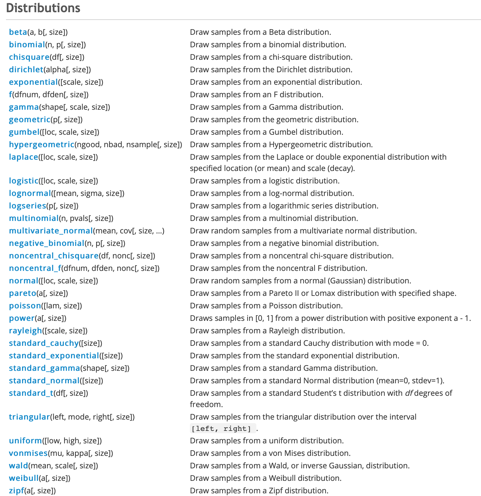
Samples of random numbers can be drawn from a variety of probability distributions. The complete list of such functions is listed under Distributions section of the numpy.random reference guide but for the purposes of the assignment I am looking at the following 5 of distribution functions.
Numpy Random Distribution Functions
- The Normal (Gaussian) Distribution Function
- The Standard Normal distribution function
- The Uniform Distribution function
- The Binomial Distribution function
- The Poisson Distribution Function
Each of the numpy.random distribution functions generate different random numbers according to different probabilities over different intervals and can be used to simulate and understand data. There are specific applications and uses for each type of distribution. However the distributions can nearly all be related to each other or transformed into each other in some way or other.
A probability distribution specifies each possible value that a random variable can assume with its probability of occurring. A random variable is any quantity that is assumed to have a probability distribution. Probability is a mathematical expression of uncertainty of the chance of a random variable taking on particular values. There are many different patterns of probability and random numbers can be drawn from various probability distributions.
A discrete random variable is one where its set of possible values is a collection of isolated points on the number line - it has a finite set of specific outcomes, while a continuous random variable is one where its set of possible values is an entire interval on the number line. Discrete random variables almost always come from counting while continuous random variables mostly come from measurement.
Probability distributions are used widely in statistical analysis, data analytics and machine learning. Probability distributions can be simulated based on their mathematical properties. Probability distributions are derived from variance or uncertainty and show which outcomes are more likely and which are less likely.
The probability distribution of a discrete random variable is often known as a probability function or a probability mass function while the probability distribution for a continuous random variable often called a mathematical a probability density function, a frequency function or a probability distribution. Probability distributions can be shown as a formula, a table or a graph.
A Probability Mass Function (PMF) returns the probability of a given outcome while a Cumulative Distribution Function (CDF) returns the probability of a value less than or equal to a given outcome and a Percent-Point Function (PPF) returns a discrete value that is less than or equal to the given probability.
If you can define a probability distribution for a dataset you are interested in, you can use the known properties of the distribution to investigate and summarise the data using statistics, plot the data and look at predicting future outcomes.
If you are interested in measurements of a population but it is not practical to measure this parameter, you could take representative samples from the population and get the average of the samples instead. A statistic is a good estimator for a population parameter and measure estimates of population parameters in a sample.
There are many ways to take samples from a population and when you calculate the average of an individual sample it is unlikely to be the actual true average for the population. You could take samples of a sample size from the population and repeat this process a number of times. NumPy random distribution functions can be used to imitate this process by simulating many many samples of a set sample size from a distribution such as the normal distribution. The mean and standard deviations from the samples can then be used to get the sampling distribution of the mean. While some random samples may have randomly big or randomly small values, overall you could take the average from each of the samples and relate these to the mean of the overall population you took them from.
Some distributions such as the normal and binomial distributions show a central tendancy around a mean value while others such as the uniform distribution do not show any preference for any one value over another and the values can be spread out anywhere in the range. Some distributions start to resemble the normal distribution under certain conditions such as when the number of samples is very large and therefore the normal distribution can be used as an approximation.
Some distributions such as the normal and binomial distributions show a central tendancy around a mean value while others such as the uniform distribution do not show any preference for any one value over another and the values can be spread out anywhere in the range.
According to machinelearningmastery.com
The two types of discrete random variables most commonly used in machine learning are binary and categorical. The most common discrete probability distributions are the Bernoulli and Multinoulli distributions for binary and categorical discrete random variables respectively, and the Binomial and Multinomial distributions that generalize each to multiple independent trials.
- A binary random variable is a discrete random variable where the finite set of outcomes is in {0, 1}.
- A categorical random variable is a discrete random variable where the finite set of outcomes is in {1, 2, …, K}, where K is the total number of unique outcomes.
(wolfram mathworld, stattrek.com and Wikipedia are good sources for information on probability distributions)
There are many plotting functions in Python libraries such as matplotlib.pyplot and seaborn.
Seaborns distplot is a very convenient way to draw a univariate distribution. It draws a histogram and fits a kernel density estimate. A histogram represents the distribution of one-dimensional data by cutting the data into ranges called bins and shows the number of values in each bin which gives a picture of how the values are distributed and the range in which the most common values fall. The kernel density estimate (kde) plots the shape of a distribution. A kde plot encodes the density of observations on one axis with height on the other axis.
The numpy.random distribution functions take various arguments but location for the centre or mean of the distribution, size for the number of samples and scale for the spread or standard deviation are some commonly used arguments.
The numpy.random.normal() function generates random numbers in a bell shaped curve centred around zero. The numbers near the centre of the distribution have a higher chance of being randomly generated while the numbers further away the centre (at zero) have less chance of being randomly generated. The numpy.random.uniform() function generates numbers between a start and finish point where any one number is as likely to occur as any other number. In a uniform distribution, you would expect to see a fairly straight line at the top while the normal distribution is bell shaped.
($\mu$ is the mean, $\sigma$ is the standard deviation which is the square root of the standard deviation, $\sigma^2$.)
Numpy.Random Distribution Functions.
The Normal (Gaussian) Distribution Function
The numpy.random.normal(loc=0.0, scale=1.0, size=None) function is used to draw random samples from a normal (Gaussian) distribution which has a symmetric, bell shaped density curve density curve described by its mean $mu$ and standard deviation $\sigma$.
The normal distribution is considered one of the most important probability distribution for a continuous random variable. It has a symmetric, bell shaped density curve. It is not one distribution but a family of distributions depending on the value of its mean $\mu$ and standard deviation $\sigma$. The normal distributions occurs often in nature. It describes the commonly occurring distribution of samples influenced by a large number of tiny, random disturbances, each with its own unique distribution. All the small influences add up to get a normal distribution.
According to wolfram mathworld
normal distributions have many convenient properties, so random variates with unknown distributions are often assumed to be normal, especially in physics and astronomy. Although this can be a dangerous assumption, it is often a good approximation due to a surprising result known as the central limit theorem. This theorem states that the mean of any set of variates with any distribution having a finite mean and variance tends to the normal distribution. Many common attributes such as test scores, height, etc., follow roughly normal distributions, with few members at the high and low ends and many in the middle.
Any distribution where the mean, median and mode of the distribution coincides is a Normal distribution. Half of the values are to the left of the centre and half to the right.
A normally distributed random variable x can be denoted as follows: x~ $N(\mu,\sigma^2)$ which means that x is normally distributed with a mean of $\mu$ and a variance of $\sigma^2$.
While all values of a normal distribution have a zero probability as it is a continuous distribution, the mean can be thought of as the centre of the distribution or where the values are more likely to be from and its standard deviation shows how likely a value is to be away from the mean value.
The density curve is symmetrical and centered about its mean. The spread is determined by the standard deviation. The data points near the centre of the distribution have a higher chance of being randomly generated while the numbers further away from the centre of the distribution have less chance of being randomly generated. Data close to the mean occur more frequently than data points further away from the mean.
numpy.random.normal distribution function
The numpy.random.normal function generates random number in a bell shaped curve centred around zero but spread out according to the scale parameter. The function depends on two factors, the mean and the standard deviation.
To use the numpy.random.normal function, the loc argument is used to specify the mean or the centre of the distribution, the scale is used to specify the standard deviation of the distribution and the size is the number of random variables to sample. Otherwise the loc or mean defaults to 0 and scale or standard deviation defaults to 1 which is the same as the Standard Normal Distribution. See below.
The mean of the distribution determines the location of the centre of the plot, while the standard deviation determines the height and shape of the graph. A larger standard deviation will result in a shorter and wider curve while a smaller standard deviation results in a tall and narrow curve.
If you supply three arguments, the first is taken to be the mean $\mu$, the second to be the scale or standard deviations $\sigma^2$ and the last to be the number of data points.
Examples of using the normal distribution function
Below is a plot of 4 normal distribution functions using different values for the loc and scale parameters for the mean and standard deviation of the distribution. This plot shows the distinctive bell shaped curve, which is taller and narrower for the distribution with the smaller standard deviation or spread and wider and flatter for the distribution with the larger standard deviation as the scale parameter. In each case the curve is centred around the mean of the distribution as the loc parameter.
Plotting the Normal Distribution function
Comparing the distribution of two normally distributed variables with different means and standard deviations.
Plotting normal distributions with various means and spreads.
Here I plot different normal distributions with various means and standard deviations.
np.random.normal # <function RandomState.normal>
# Generate some random datasets using random.normal
loc,scale,size = 5,1,3000

sample1 = np.random.normal(loc,scale,size)
sample2 = np.random.normal(loc+1, scale,size)
sample3 = np.random.normal(loc-1,scale+1.5,size)
sample4 = np.random.normal(loc-1,scale-0.2, 3000)

# set up the plot figure
plt.figure(figsize=(12,4))  # set the size of the figure
# using seaborn distplot functions to plot given loc(mean) and scale(standard deviation)
sns.distplot(sample1,label="$\mu=5,\ \sigma=1$")
sns.distplot(sample2, label ="$\mu=6,\ \sigma=1$")
sns.distplot(sample3, label="$\mu=4,\ \sigma=2.5$")
sns.distplot(sample4, label ="$\mu=4,\ \sigma=0.8$")
plt.legend(loc="best")
plt.ylim([-0.05, 0.6]) # set the plot limits on the y-axis
plt.suptitle('Normal Distribution with various $\mu$ and $\sigma$')
plt.grid(True)

Verifying the mean and the standard deviation.
The mean is an estimator of the centre of the distribution. The median is another estimator for the centre of the distribution. It is the value where half of the observatins are below and half are above it. The median is not sensitive to the tails of the distribution and is considered robust.
print('The means of the distributions are \n sample1: %.3f, sample2: %.3f, sample3: %.3f and sample 4:%.3f' % (np.mean(sample1), np.mean(sample2),np.mean(sample3),np.mean(sample4)))
print('The medians of the distributions are \n sample1: %.3f, sample2: %.3f, sample3: %.3f and sample 4:%.3f' % (np.median(sample1), np.median(sample2),np.median(sample3),np.median(sample4)))
print('The standard deviations of the distributions are \n sample1: %.3f, sample2: %.3f, sample3: %.3f and sample 4:%.3f' % (np.std(sample1), np.std(sample2),np.std(sample3),np.std(sample4)))
The plots above demonstrate the bell-shaped nature of the distributions. Changing the loc parameter for the mean will move the curve along the x-axis while changing the scale parameter result in wider or narrower curves.
There is a general rule that 68.27% of the values under the curve fall between -1 and +1 standard deviations from the mean or centre, 95.45% under the curve between -2 and 2 standard deviations and 99.73% between -3 and 3 standard deviations. This rule applies no matter what the mean and standard deviations are. For any normally distributed variable, irrespective of it's mean and standard deviation, if you start at the mean and move one standard deviation out in any direction, the probability of getting a measurement of value from this variable within this range is just over 68%, the probability of getting a value within two standard deviations is over 95% and the probability of getting a value within 3 standard deviations from the mean is 99.73%. This leaves a very small percentage of values that lie further than 3 standard deviations from the mean.
The curves do not not actually cross the x-axis at all as it goes to infinity in both directions of the mean. However the chances of observing values more than 3 standard deviations from the centre or mean of the curve is very small.
All the plots above are normally distributed but with different means $\mu$ and standard deviations $\sigma$. A normal distribution with a mean of 0 and a standard deviation of 1 is a special case of the normal distribution which brings me to the next distribution - the Standard Normal Distribution.
The Standard Normal Distribution function
For an approximately normal data set, almost 68% of the data points fall within one standard deviation from the mean, while 95% of the data falls within 2 standard deviations and 99.7% fall within 3 standard deviations.
There are many different normal distributions with different means and variances which would have made them difficult to have been tabulated in the statistical tables. The standard normal distribution is a special case of the normal distribution with $\mu$ of 0 and standard deviation $\sigma$ of 1 and this is tabulated and can be used to find the probabilities for any normal distribution. All questions regarding the normal distribution can be converted into questions regarding the standard normal distribution.
The standard normal distribution is a special case of the normal distribution.
It is the distribution that occurs when a normal random variable has a mean of zero and a standard deviation of one. The normal random variable of a standard normal distribution is called a standard score or a z score. Every normal random variable X can be transformed into a z score.
The numpy.random.standard_normal distribution function is used to draw samples from a Standard Normal distribution that has a mean of 0 and a standard deviation of 1. The standard normal distribution, of the random variable z, has $\mu$ = 0 and $/sigma$ = 1 and can be used to calculate areas under any normal distribution. z~ $N(0,1)$
To use this numpy.random.standard_normal function, you just need to supply the number of data points to generate as the size argument. Without specifying the number of data points you will just get a single value.
Note that the numpy.random.randn() function in the section on simple random data functions a convenience function for numpy.random.standard_normal. It returns a single float or an ndarray of floats. See numpy.random.randn.
np.random.standard_normal # <function RandomState.standard_normal>
# Generate some random samples from standard normal distributions

sample1 = np.random.standard_normal(100) # only need to set the size of the samples
sample2 = np.random.standard_normal(500)
sample3 = np.random.standard_normal(1000)
sample4 = np.random.standard_normal(2000)
# set up the plot figure size

plt.figure(figsize=(12,4))
# using seaborn kdeplot functions to plot
sns.kdeplot(sample1,shade=True,label="size=100")
sns.kdeplot(sample2, shade=True,label ="size=500")
sns.kdeplot(sample3, shade=True,label ="size=1000")
sns.kdeplot(sample4, shade=True,label ="size=2000")

plt.legend(loc="best") # set the legends
plt.suptitle('The Standard Normal Distribution with various $\mu$ and $\sigma$') # the title of the plot
plt.grid(True)
plt.ylim([-0.05, 0.5]) # set the plot limits on the y-axis
print('The means of the distributions are \n sample1: %.3f, sample2: %.3f, sample3: %.3f and sample 4:%.3f' % (np.mean(sample1), np.mean(sample2),np.mean(sample3),np.mean(sample4)))
print('The medians of the distributions are \n sample1: %.3f, sample2: %.3f, sample3: %.3f and sample 4:%.3f' % (np.median(sample1), np.median(sample2),np.median(sample3),np.median(sample4)))
print('The standard deviations of the distributions are \n sample1: %.3f, sample2: %.3f, sample3: %.3f and sample 4:%.3f' % (np.std(sample1), np.std(sample2),np.std(sample3),np.std(sample4)))
print("\n")

The above plots show that whatever the number of values generated, the curve is always centred about the mean of 0, most of the values are clustered around the centre and most of the values are within 2 standard deviations of the mean. As the size of the sample increases, the shape becomes more symetrical.
The Uniform distribution functions.
The continuous Uniform distribution function is one of the simplest probability distributions where all it's possible outcomes are equally likely to occur. It has constant or uniform probability.
Wikipedia describes the Uniform Distribution) as the continuous uniform distribution or rectangular distribution is a family of symmetric probability distributions such that for each member of the family, all intervals of the same length on the distribution's support are equally probable. The support is defined by the two parameters, a and b, which are its minimum and maximum values.
The continuous uniform distribution takes values in the specified range (a,b). The curve describing the distribution is rectangle shaped because any interval of numbers has the same probability of being drawn as any other interval of the same width. Each interval has constant height across it and 0 everywhere else. The area under the curve must be equal to 1 and therefore the height of the curve equals $\frac{1}{b-a}$. The probability density function of a uniformly distributed variable x is $f(x)= \frac{1}{a-b}$ if $a<=x<=b$ or zero otherwise.
The expected value of the uniform distribution is $\frac{b+a}{2}$ the midpoint of the interval and the variance $\sigma^2$ is $\frac{1}{12}(b-a)^2$.
When the interval is between 0 and 1, it is known as the Standard Uniform distribution. The Standard Uniform distribution, where a is 0 and b is 1 is very commonly used for random number generation and in statistics in general. The expected value of the standard uniform distribution is $\frac{1}{2}$ and the variance is $\frac{1}{12}$.
As all outcomes are equally likely there is no one particular value that occurs more frequently than any other and therefore there is no skew in a uniform distribution like there is in other distributions.
The uniform distribution can be used to generate random numbers between a minimum and a maximum value where each number is equally likely to occur. Rolling a dice several times is an example of the uniform distribution, where each number on the dice is equally likely to occur on each roll. No single side of the dice has a higher chance than another.
While many natural things in the world have approximately normal distributions where values are more likely to fall in the centre of the distribution, a uniform distribution can be used for modeling events that are equally likely to happen in a given interval between a minimum and a maximum range. This minimum value is usually referred to as a while the maximum value is referred to as b.
If a random variable is uniformly distributed between a minimum (a) and maximum value (b), then the distribution can be used to calculate the probability that a value will lie in a cetain part of the interval, say between two points c and d where d > c. The probability for something in such an interval is calculated using $\frac{d-c}{b-a}$.
The numpy.random.uniform function.
numpy.random.uniform(low=0.0, high=1.0, size=None
Samples are uniformly distributed over the half-open interval $[low, high)$ (includes low, but excludes high). In other words, any value within the given interval is equally likely to be drawn by uniform.
To use this function, you provide the lower $low$ and upper $high$ bounds of the interval to specify the minimum (a) and maximum (b) possible values in the range. The smaller number provided will be taken as the lower bounds and the bigger number as the upper bound. Without providing an interval bounds, the function assumes a standard uniform distribution.
The function randomly samples from the uniform distribution over the specified interval. If not argument at all is provided then it will return a single value in the interval $[0.0,1.0)$. If a single value is provided to the function, a single value will be returned from the interval between 0 and that number. If two values are provided, then a single value will be returned from the interval between between these two numbers. A third value provided will be used as the size of the array returned.
The simple numpy.random.rand function in section 2 also returns samples from the continuous uniform distribution but only in the $[0.0, 1.0)$ interval. The other numpy.random functions random_sample,random, sample and ranf can be used to sample from $[a,b)$ intervals other than between 0 and 1 by multiplying the output by $(b-a)$ and adding $a$ but the numpy.random.uniform function is easier to use for this purpose.
Sampling from the continuous uniform distribution
The following are examples of using the numpy.random.uniform function where various numbers of arguments are provided as outlined above.
np.random.uniform() # returns a single random value in the interval [0,1)
np.random.uniform(5) # returns a single value from the interval $[0,5)$
np.random.uniform(5,10) # returns a single value in the interval [6,10)]
np.random.uniform(5,10,15) # returns an array of 15 values from the interval [5,10)
Here I show that the mean and median values are very close, while the mean is the midpoint of the interval and the variance is equal to $\frac{1}{12}(b-a)^2$. If the size of the sample is changed in the code below, the mean and median get closer and closer to each other and to the expected value. These results are the same no matter what interval $[a,b)$ is used. Also showing that all the values are from the interval $[a,b)$
np.random.uniform #<function RandomState.uniform>
a,b,size = 5,10,500

x = np.random.uniform(a,b,size) # returns an array of 500 values from the interval [5,10)
print(x)
print('\n Expected value is %.3f, Variance: %.3f' % ((b+a)/2, ((b-a)**2)/12))
print('The mean is %.3f, the median is %.3f' % (np.mean(x), np.median(x)))

# Checking that all the values are within the given interval:
print(np.all(x >= a))

print(np.all(x < b))
Using the same random.seed to show the similarity between the numpy.random.uniform is similar to numpy.random.random
# 100 values from the uniform 2,11] interval
np.random.seed(1)
u1 = np.random.uniform(2,11,100)
np.random.seed(1)
u2 =(b-a)* np.random.random((100)) +a
u1 ==u2
Plotting Uniform distributions
# generate random sample of 1000 from two different intervals

a,b, size = -20,20,1000 # set the a,b and size parameters
u1 = np.random.uniform(a,b,size)  # sample from -20,20 interval
u2 = np.random.uniform(a+30, b+30, size)# sample from -10,50 interval

plt.figure(figsize=(12,4)) # set up the figure size for the plot

ax = sns.distplot(u1, bins=100, label="$[-50,50)$");  # distplot using 100 bins
ax = sns.distplot(u2, bins=100, label="$[-20,80)$");

ax.set(xlabel="Uniform Distribution", ylabel ="Frequency")  # set the x-axis and y-axis labels
plt.legend() #
plt.suptitle("The Uniform Distribution over overlapping intervals")
plt.ylim([-0.005,0.05])
print('The mean of u1 is %.3f' % np.mean(u1)) # to 3 decimal places
print('The mean of u2 is %.3f' % np.mean(u2)) # to 3 decimal places

Plotting samples of size 1000 from continuous uniform distributions across various interval using matplotlib plots
Also showing the means which can be seen as the midpoint of the intervals for each distribution.
Using the example then from themanual to plot a histogram of a uniform distribution function and its probability density function using the np.ones_like function. The area under the curve between a and b is 1
# create samples from uniform distribution over different intervals but the same size
x1 = np.random.uniform(2,12,1000)
x2 = np.random.uniform(5,20,1000)
x3 = np.random.uniform(2,20,1000)
x4 = np.random.uniform(-5,5,1000)

plt.figure(figsize=(12, 3)) # set up the figure
plt.subplot(141) # select 1st of 4 plots
plt.hist(x1) # plot first sample x1
plt.subplot(142) # select 2nd of 4 plots
plt.hist(x2) # plot second sample x2
plt.subplot(143)
plt.hist(x3)
plt.subplot(144)
plt.hist(x4)
plt.suptitle('Uniform Distribution over various intervals')
plt.show()
print('The means of these distributions are for x1: %.3f, x2: %.3f, x3: %.3f and x4: %.3f' %(np.mean(x1), np.mean(x2), np.mean(x3), np.mean(x4))) # to 3 decimal places

# Example from the numpy.random.uniform reference manual
#Display the histogram of the samples, along with the probability density function:
s = np.random.uniform(-1,0,1000)
# use np.ones_like function to return an array of ones with the same shape and type as s.
import matplotlib.pyplot as plt

count, bins, ignored = plt.hist(s, 15, density=True) # use 15 bins
plt.plot(bins, np.ones_like(bins), linewidth=2, color='r') ## add a horizontal line at 1.0 using the np.ones like
plt.show()

The Binomial Distribution
The numpy.random.binomial function is used to draw samples from a Binomial Distribution which is considered one of the most important probability distributions for discrete random variables. The Binomial distribution is the probability distribution of a sequence of experiments where each experiment produces a binary outcome and where each of the outcomes is independent of all the others.
The binomial distribution is the probability of a success or failure outcome in an experiment that is repeated many times. A binomial experiment has only two (bi) possible outcomes such as heads or tails, true or false, win or lose, class a or class b etc. One of these outcomes can be called a success and the other a failure. The probability of success is the same on every trial A single coin flip is an example of an experiment with a binary outcome.
According to mathworld.wolfram, the Binomial Distribution gives the discrete probability distribution $P_p(n|N)$ of obtaining exactly n successes out of N Bernoulli trials (where the result of each Bernoulli trial is true with probability $p$ and false with probability $q=1-p$). See also https://en.wikipedia.org/wiki/Binomial_distribution.
The results from performing the same set of experiments, such as repeatedly flipping a coin a number of times and the number of heads observed across all the sets of experiments follows the binomial distribution.
$n$ is usually used to denote the number of times the experiment is run while $p$ is used to denote the probability of a specific outcome such as heads.
A Bernoulli trial is a random experiment with exactly two possible outcomes, success and failure, where probability of success is the same every time the experiment is conducted. A Bernoulli process is the repetition of multiple independent Bernoulli trials and it's outcomes follow a Binomial distribution. The Bernoulli distribution can be considered as a Binomial distribution with a single trial (n=1).
A binomial experiment consists of a number $n$ of repeated identical Bernoulli trials
- where there are only two possible outcomes, success or failure
- the probability of success $p$ is constant (the same in every trial)
- the $n$ trials are independent - outcome of one trial does not affect the outcome of another trial.
- The binomial random variable $x$ is the number of successes in $n$ trials.
The outcome of a binomial experiment is a binomial random variable. Binomial probability is the probability that a binomial random variable assumes a specific value. -b(x,n,P): Binomial probability - the probability that an n-trial binomial experiment results in exactly x successes.
The binomial distribution has the following properties:
- The mean of the distribution is equal to $n*P$
- The variance $\sigma^2$ is $n*P*(1-p)$
- the standard deviation $sqrt(n*P*(1-p))$
Some other properties of the Binomial Distribution from Wikipedia:
- In general, if
npis an integer, then the mean, median, and mode coincide and equalnp. - The Bernoulli distribution is a special case of the binomial distribution, where n = 1.
- The binomial distribution is a special case of the Poisson binomial distribution, or general binomial distribution, which is the distribution of a sum of n independent non-identical Bernoulli trials B(pi)
- If n is large enough, then the skew of the distribution is not too great. In this case a reasonable approximation to B(n, p) is given by the normal distribution
- The binomial distribution converges towards the Poisson distribution as the number of trials goes to infinity while the product np remains fixed or at least p tends to zero. Therefore, the Poisson distribution with parameter λ = np can be used as an approximation to B(n, p) of the binomial distribution if n is sufficiently large and p is sufficiently small. According to two rules of thumb, this approximation is good if n ≥ 20 and p ≤ 0.05, or if n ≥ 100 and np ≤ 10.[
Using the numpy.random.binomial function
The numpy.random.binomial function is used to sample from a binomial distribution given the number of trials $n$ and the probability $p$ of success on each trail. The number of samples $size$ represents the number of times to repeat the $n$ trials.
This function takes an integer to set the number of trials which must be greater than or equal to zero. The probability must be in the interval $0,1]$ as total probability always sums to one. It returns an array of samples drawn from the binomial distribution based on the $n$ and $p$ and $size$ parameters given to the function. Each sample returned is equal to the number of successes over n trials.
The np.random.binomial(n, p) function can be used to simulate the result of a single sequence of n experiments (where n could be any positive integer), do so using using a binomially distributed random variable.
For example to find the probability of getting 4 heads with 10 coin flips, simulate 10,000 runs where each run has 10 coin flips. This repeats the 10 coin toss 10,000 times.
Example of drawing samples from a binomial distribution.
Draw samples from a distribution using np.random.binomial(n, p, size) where:
- $n$ the number of trials,
- $p$ the probability of success in each trial
- $size$ is the number of samples drawn (the number of times the experiment is run)
np.random.binomial # <function RandomState.binomial>
n, p = 10, .5  # number of trials, probability of each trial
s = np.random.binomial(n, p, 100)
print(s)  ## returns an array of 100 samples
print(np.size(s))
This returns a numpy array with 100 (size=100) samples drawn from a binomial distribution where the probability of success in each trial is 0.5 (p=0.5), where each number or sample returned represents the number of successes in each experiment which consist of 10 bernoulli trials (n=10)
These 100 number represents the number of successes in each experiment where each experiment consists of 10 bernoulli trials each with 0.5 probability of success.
[ 8 10 2 ... 6 5 5]
8 out of 10 successes in the first experiment of 10 trials, 10 successes in the second experiment of 10 trials, 2 out of 10 successes in the third experiment of 10 trials etc..
Plotting the Binomial distribution
Here I am using seaborn to plot a Binomial distribution that has 100 trials in each experiment, the probability of success in each trial is 0.9 and the number of samples (or times the experiment is run) is 1000. As the plot shows, the distribution is skewed to the right because the probability of success in each trial is 0.9 so more samples will have more successes. When the probability of success is less than 0.5 then a left skewed distribution is expected. The probability of success probability determines the skew. A probability of 0.5 would have a centred distribution.
If n is large enough, then the skew of the distribution is not as great and as mentioned above, a reasonable approximation to B(n, p) is given by the normal distribution.). When I increase the number of trials by multiples while keeping the same probability the skew becomes lesser and the curve looks more 'normal'.
sns.set_style('darkgrid')
n,p,size = 20, 0.9, 1000 # # number of trials, probability of success in each trial, number of samples (experiments run)
# Generate a random datasets using random.binomial
np.random.seed(10)
b11 = np.random.binomial(n, p, size) # p= 0.1
b22 = np.random.binomial(n*5, p, size) # p= 0.3

# Set up the matplotlib figure
f,axes = plt.subplots(2,1,figsize=(10,7),sharex=False)

sns.distplot(b11, label="p=0.1", kde=False,color="r",ax=axes[0]) # p=0.1
sns.distplot(b22, label="p=0.3", kde=False, color="g",ax=axes[1]) # p=0.5
plt.suptitle("Binomial Distributions with different numbers of trials $n$")

plt.show()

Plotting the binomial distribution with various probabilities.
Below I plot binomial distribution with increasing probabilities. The bottom left curve with probabilites of 0.5 is centred while the sample with lower probability is right skewed and the samples with probabilites closer to 1 are left skewed.
# Set up the matplotlib figure

sns.set_style('darkgrid')
n,p,size = 20, 0.1, 1000 # # number of trials, probability of success in each trial, number of samples (experiments run)
# Generate a random datasets using random.binomial

b1 = np.random.binomial(n, p, size) # p= 0.1
b2 = np.random.binomial(n, p+0.2, size) # p= 0.3
b3= np.random.binomial(n, p+0.4, size) # p= 0.5
b4= np.random.binomial(n, p+0.8, size) # p= 0.9

# Set up the matplotlib figure
f,axes = plt.subplots(2,2,figsize=(10,7),sharex=False)

sns.distplot(b1, label="p=0.1", kde=False, color="r",ax=axes[0,0]) # p=0.1
sns.distplot(b2, label="p=0.3", kde=False, color="g",ax=axes[0,1]) # p=0.5
sns.distplot(b3 ,label="p=0.5", kde=False, color="m",ax=axes[1,0]) # p=0.9
sns.distplot(b4 ,label="p=0.9", kde=False, ax=axes[1,1]) # p=0.9


plt.suptitle("Binomial Distributions with different probabilities $p$")
ax.set(xlabel="Binomial Distribution", ylabel ="Frequency")

plt.show()

print('The means of these distributions are for b1: %.3f, b2: %.3f, b3: %.3f and b4: %.3f' %(np.mean(b1), np.mean(b2), np.mean(b3), np.mean(b4))) # to 3 decim
looking at the statistics: mean, median, mode, variance and standard deviation
Here I check that the mean of the distribution is equal to $n*P$ and that the standard deviation is equal to $sqrt(n*P*(1-p))$. In general, if np is an integer, then the mean, median, and mode coincide and equal np. This is shown below where the mean, median and mode are very similar and equal to n times p.
There seems to be no mode function in numpy but there is one in the scipy.stats package which I use here.
n,p,size = 30, 0.3, 10000 # # number of trials, probability of success in each trial, number of samples (experiments run)
# Generate a random datasets using random.binomial

s1 = np.random.binomial(n, p, size) # p= 0.3

from scipy import stats # no mode in numpy
print('Mean: %.3f'% np.mean(s1), 'Median: %.3f' % np.median(s1),'Standard Deviation: %.3f' % np.std(s1))

print('n times p : %.3f'% (n*p))
print('np.sqrt(n*p*(1-p)) %.3f' %np.sqrt(n*p*(1-p)))
stats.mode(s1)
Example of using numpy.random.binomial
The numpy random reference docs demonstrates the following real world example.
A company drills 9 wild-cat oil exploration wells, each with an estimated probability of success of 0.1. All nine wells fail. What is the probability of that happening? To do this, 20,000 trials of the model are simulated and then the number generating zero positive results are counted where n = 9, p = 0.1 and size = 20,000
Below I use the example and expand on it:
# set the parameters and create a sample, then check how many trials resulted in zero wells succeeding
n,p,size = 9, 0.1, 20000
s =np.random.binomial(n, p, size)
print(sum(s == 0)/20000.) # what is probability of all 9 wells failing.
This shows that there is a 39% probability of all 9 wells failing (0 succeeding) but I could also check the probability of all 9 being successful which is 0. The distribution plot shows the probabilities for each possible outcome. Below I use a lambda function to check for the probability for 0,1,2 .. up to all the 9 wells being successful. This corresponds with the plot below which shows that no well succeeding or only 1 well succeeding have the highest probabilites. The probabilites of more than two wells succeeding given p=0.1 is very small and the probabilities of more than two successful wells is very very small.
print(sum(s == 0)/20000.) # what is probability of all 9 wells failing.
print(sum(s == 9)/20000.) # probability of all 9 successeding
print(sum(s == 1)/20000.) #probability of 1 well being successful
Write a lambda function to check the probabilties of 0,1,2,3.. up to all 9 wells failing.
n,p,size = 9, 0.1, 20000 ## set the probability of success, number of bernouilli trials and number of samples or experiments
g = lambda x: sum(np.random.binomial(n,p,size)==x)/size #

[g(i) for i in range(10)] ## run the lambda function g to get the probabilities for the numbers in the range 0 to 9
[np.mean(g(i)) for i in range(10)] # get the average
sns.distplot(s)

If the probabiility is p=0.3 with n=10 trials in each experiment then the expected number of successful outcomes is 3 out of 10 trials in each experiment.
The Binomial distribution summarizes the number of successes k in a given number of Bernoulli trials n, with a given probability of success for each trial p.
The examples on machinelearningmastery show how to simulate the Bernoulli process with randomly generated cases and count the number of successes over the given number of trials using the binomial() NumPy function. However these examples also make use of the scipy-stats-binom function but I will use these as a basis for an example using numpy.random.binomial function.
This numpy.random.binomial function takes the total number of trials and probability of success as arguments and returns the number of successful outcomes across the trials for one simulation.
- With n of 100 and p of 0.3 we would expect 30 cases to be successful.
- Can calculate the expected value (mean) and variance of this distribution.
n,p,size = 100, 0.3, 1000 ## set the probability of success, number of bernouilli trials and number of samples or experiments
s3 = np.random.binomial(100, 0.3, 1000)
plt.figure(figsize=(10,4))
sns.distplot(s3)
print(np.mean(s3))

# example of simulating a binomial process and counting success
import numpy as np
# define the parameters of the distribution
n,p = 100, 0.3
# run a single simulation
success = np.random.binomial(n, p)
print('Total Success: %d' % success)
# 2
print('Mean=%.3f, Variance=%.3f' % (np.mean(success), np.var(success)))
Calculate the probaility of so many successes in every 100 trials. Do this in steps of 10. This shows that as expected, 30 successful outcomes has the highest probability.
n,p,size = 100, 0.3, 10000 ## set the probability of success, number of bernouilli trials and number of samples or experiments
g = lambda x: sum(np.random.binomial(n,p,size)==x)/size*100 #
[g(i) for i in range(10,110,10)] ## run the lambda function g to get the probabilities for the numbers in the range 0 to 9
n,p=100,0.3

for x in range(10,110,10):  # go up in steps of 10
    success =np.random.binomial(n, p) ## calculate the number of successes
    print('probability of ',x,'successes in ',n, 'trials is', sum(np.random.binomial(n,p,size)==x)/100,'%')
The Poisson Distribution function
The numpy.random.poisson function is used to draw samples from a Poisson distribution. It takes a $\lambda$ parameter as well as a size for the number of samples.
numpy.random.poisson(lam=1.0, size=None)
The Poisson distribution is the limit of the binomial distribution for large N.
The Poisson distribution, named after French mathematician Siméon Denis Poisson, is a discrete probability distribution that expresses the probability of a given number of events occurring in a fixed interval of time or space if these events occur with a known constant rate and independently of the time since the last event. The Poisson distribution can also be used for the number of events in other specified intervals such as distance, area or volume.
It was originally developed in France in the 1830's to look at the pattern of wrongful convictions in a year. A poisson distribution gives the probability of a number of events in an interval generated by a Poisson process which is a model for describing randomly occuring events. It is defined by the rate parameter, $\lambda$, which is the expected number of events in the interval.
A poisson random variable can be used to model the number of times an event happened in a time interval. A poisson distribution is the probability distribution of independent occurences of an event in an interval. It can be used for finding the probability of a number of events in a time period, or the probability of waiting some time until the next event occurs. When you know how often an event has occurred then you can it to predict the probability of such events happening.
The poisson probability distribution function takes one parameter which is lamda $\lambda$ or the rate parameter which is a function of both the average events per time and the length of the time period or the expected number of events in an interval. It can be used for count based distributions where the events happen with a known average rate and independently of time since the last event such as the number of times an event occurs in an interval of time or space such as number of winning lottery tickets per week, the number of visitors to a website in a period, the number of patients admitted to a hospital A&E in a particular hour, the number of goals scored by a team in a match etc.
An event can occur 0, 1, 2, ... times in an interval. The average number of events in an interval is designated $\lambda$ which is the event rate known as the rate parameter. To find the probability of observing $k$ events in an interval you use the following formula:
$${\displaystyle P(k{\text{ events in interval}})={\frac {\lambda ^{k}e^{-\lambda }}{k!}}}$$where $\lambda$ is the average number of events per interval, $e$ is the number 2.71828 (which is the base of the natural logarithms), $k$ takes values 0, 1, 2, ... $k! = k * (k − 1) * (k − 2) * ... * 2 * 1 $is the factorial of k.
As the rate parameter $\lambda$ is changed, the probability of seeing different numbers of events in one interval is changed. The most likely number of events in the interval for each curve is the rate parameter which is the only number needed to define the Poisson distribution. (As it is a product of events/interval and the interval length it can be changed by adjusting the number of events per interval or by adjusting the interval length).
If you give the numpy.random.poisson function the mean or average number of occurances as $\lambda$, it returns the probability that $k$ number of events will occur.
The default settings is $\lambda$ = 1 and generate a single value.
(lam=1.0, size=None)
If you supply a rate parameter of 5 to the numpy.random.poisson function it will randomly generates numbers from 0,1,2,3 up to infinity but the most likely number to occur will be 5, followed by the numbers closer to 5 such as 3 and 4.
You can also specify how many samples to generate if you want more than a single number.
Using the numpy.random.poisson function.
Starting off with the example from the documentation, set $\lambda$ to 1 and draw 1000 values from a poisson distribution that has a rate of 5.
np.random.poisson # <function RandomState.poisson>
import numpy as np  # from documentation
plt.figure(figsize=(8,4)) # set the figure size
s = np.random.poisson(5, 1000) # lambda 5, 1000 samples
import matplotlib.pyplot as plt
count, bins, ignored = plt.hist(s, 14, density=True) # plot histogram of values
plt.show()

Draw values from poisson distributions with different $\lambda$ values
Here I will draw samples from poisson distributions with different rate parameters in a 10 by 5 array. Create a DataFrame and then look at the summary statistics using the pandas.describe function. The expected value, variance and lambda should all be very close.
# Draw each 10 values for lambda 5,10,15,20 and 50
s = np.random.poisson(lam=(5, 10,15,20,50), size=(1000, 5))
import pandas as pd
poissondf= pd.DataFrame(s, columns=['lambda=5','lambda10','lambda=15','lambda=20','lambda=50'])
print(poissondf.describe())
print("\n Variances")
print(poissondf.var())
Again drawing samples from another poisson distribution with different $\lambda$'s
The curves show the peak around the expected value equal to $\lambda$. The curve shifts depending on the mean.
# Set up the matplotlib figure

plt.figure(figsize=(8,5))
sns.set_style('white')
lam,size = 4,2000
# Generate a random datasets using random.binomial
p1 = np.random.poisson(lam, size)
p2 = np.random.poisson(lam+8, size)

sns.distplot(p1,label = "$\lambda$=4", kde=False,color="pink") #
sns.distplot(p2, label = "$\lambda$a=12", kde=False, color="skyblue") #

plt.legend()
plt.title("Poisson Distribution with different $\lambda$")
plt.show()

Showing the various distributions
size =100
sn1 = np.random.standard_normal(size)
n1 = np.random.normal(1,2,size)
u1 = np.random.uniform(1,10,size)

p1 = np.random.poisson(5, size)
b1 = np.random.binomial(10, 0.3, size)
plt.figure(figsize=(12,5)) # set up the figure size

# plotting the various distributions using kde plot, setting legends
sns.kdeplot(sn1, label ="standard_normal", shade=True) # using the kde plots and shading in
sns.kdeplot(n1, label ="normal", shade=True)
sns.kdeplot(u1, label = "uniform", shade=True)
sns.kdeplot(p1, label = "poisson", shade=True)
sns.kdeplot(b1, label = "binomial",shade=True)
plt.suptitle("Various distibution functions for same sample size")
plt.ylim([-0.01,0.5]) # set the y axis
plt.legend() # show the legends
plt.show()

size =1000
sn2 = np.random.standard_normal(size)
n2 = np.random.normal(1,2,size)
u2 = np.random.uniform(1,10,size)
p2 = np.random.poisson(5, size)
b2 = np.random.binomial(10, 0.3, size)
plt.figure(figsize=(12,5))
sns.kdeplot(sn2, label ="standard_normal",shade=True)
sns.kdeplot(n2, label ="normal",shade=True)
sns.kdeplot(u2, label = "uniform",shade=True)
sns.kdeplot(p2, label = "poisson",shade=True)
sns.kdeplot(b2, label = "binomial",shade=True)
plt.title("Various distibution functions for same sample size")
plt.legend()
plt.show()

4. Explain the use of seeds in generating pseudorandom numbers.
Pseudo-random number generators (PRNG's) and seeds
Computer programs produce outputs based on inputs and according to a set of predetermined rules. Pseudorandom numbers are generated in a sequence according to some deterministic algorithm from an input called a seed which is a number that is used to initialise the pseudorandom number generator. The seed used is typically the time in milliseconds on the computer when the code was run and is used as the starting point of the process.
According to statisticshowto, a random seed specifies the start point when a computer generates a random number. The random seed can be any number but it usually comes from seconds on the computer system's clock which counts in seconds from January 1, 1970. (known as Unix time). This ensures that the same random sequence won't be repeated unless you actually want it to.
Pseudo random number generators can be seeded which makes them deterministic. To recreate the exact same sequence of random numbers, then you can just explicitly supply the seed as an input to the random number generator. This means that while the numbers generated look random they are not truly random but pseudorandom. These pseudorandom numbers contain no real randomness at all - randomness is just being imitated - but they can take the role of random numbers for certain applications.
If you reinitialise a random number generator with the same seed, the default seed is ignored and the same sequence of pseudorandom numbers will be produced.
This all means that the outputs can be repeated by following the same set of steps and given the same inputs. Therefore if you know this seed then you can predict the next number to be generated in a sequence. Pseudorandom number generators should therefore not be used for cryptographic purposes because their predictability could be used to break the encryption but there are times when the exact same sequences of numbers may be required.
Psuedorandom numbers are suitable for purposes such as simulating datasets, testing machine learning algorithms etc as well as ensuring reproducibility of code for code sharing, teaching and demonstration purposes. Computer random number generation algorithms are based on patterns which generate numbers that follow particular probability distributions. Setting a seed will produce the same sequence of random numbers each time.
According to pynative.com
generally the seed value is the previous number generated by the generator. However, When the first time you use the random generator, there is no previous value. So by-default current system time is used as a seed value.
There are many different ways to generate pseudo-random numbers. Python uses the Mersenne Twister as the core generator. According to wikipedia, the Mersenne Twister is a pseudorandom number generator (PRNG) and is by far the most widely used general-purpose PRNG whose name derives from the fact that its period length is chosen to be a Mersenne prime (a prime number that is one less than a power of two. That is, it is a prime number of the form Mn = 2n − 1 for some integer n.).
Khan Academy has a video that gives a very good overview of how seeds are used in random number generators at Khan academy random vs pseudorandom number generators from which the following notes are based.
The physical world contans many truly random fluctuations everywhere. Truly random numbers could be generated by measuring or sampling this noise such as the electric current of tv static over time. Such random sequences could be visualised using a random walk where a path is drawn that changes direction according to each number. Random walks have no pattern at all as the next point is always unpredictable. Random processes are nondeterministic since they are impossible to determine in advance whereas machines are deterministic because their operation is predictable and repeatable. In 1946 while involved in running computations for the military, John Neumann required quick access to randomly generated numbers that could be repeated if necessary but as the computers of the time had very limited memory it could not store long random sequences. Nuemann therefore developed an algorithm to mechanically simulate the scrambling aspect of randomness as follows.
First a truly random numbers called the seed (which could come from measurement of noise or the current time in milliseconds) is selected which is then provided as input to a very simple calculation where the seed is multiplied by itself, the middle of this output becomes the seed for the next step and the process repeated as many times as required. This was called the middle-squares method and was the first pseudorandom number generator. The randomness of the sequence depends only on the randomness of the initial seed and the same seed will generate the same sequence.
The difference between a random generated versus a pseudorandomly generated sequence is that eventually the pseudorandom sequence will repeat when the algorithm reaches a seed it has previously used. There are many sequences that cannot occur in a pseudorandom sequence. The length before the pseudorandom sequence repeats is called the period and the period is strictly limited by the length of the initial seed. The longer the length of the initial seed the longer the period, so a 4 digit seed will produce a longer period of unrepeating sequences than a 3 digit seed which is will produce a longer period than a two digit seed etc.
For a pseudorandom sequence to be indistinguishable from a randomly generated sequence, it must be impractical for a computer to try all seeds and look for a match. There is an important distinction in computer science between what is possible versus what is possible in a reasonable amount of time. With pseudorandom generators the security increases as the length of the seed increases. If the most powerful computer would take hundreds of years to run through all seeds then we can safely assume its practically secure instead of perfectly secure. As computers get faster the seed size must increase accordingly.
Instead of having to share the entire random sequence in advance, you can share the relatively short random seed and expand it into the same random looking sequence when needed.
In summary, pseudorandom number generators (prngs) are algorithms for generating random looking numbers drawn from a probability distribution where the numbers are generated according to some deterministic algorithm from the input seed. The seed is the starting point for the algorithm. Different numbers used as the seed will produce a different set of pseudo random numbers from the same algorithm as they have a different starting point. If the starting point is the same and the steps in the algorithm are the same, then the outputs will be the same.
Using seeds in numpy.random
- Explain the use of seeds in generating pseudorandom numbers
According to the numpy.random.seed documentation , the numpy.random.seed(seed=None) method is called when RandomState is initialized and can be called again to re-seed the generator.
In NumPy the Mersenne Twister is the basis for NumPy pseudo-random number generator.
The numpy.random.RandomState class is the container for the Mersenne Twister pseudo-random number generator.
RandomState exposes a number of methods for generating random numbers drawn from a variety of probability distributions.
These include all the various functions mentioned above and other distribution functions not covered here.
Throughout the document I have looked at various functions and each one shows <function RandomState.function-name> when simply called without the brackets.
The random seed used to initialize the pseudo-random number generator can be any integer between 0 and 2**32 - 1 inclusive or a sequence of such integers. The default is None in which case RandomState will try to read data from /dev/urandom (or the Windows analogue) if available or seed from the clock otherwise.
/dev/urandom are special files in Unix-like operating systems that serve as pseudorandom number generators which allow access to environmental noise collected from device drivers and other sources.
The call to numpy.random.seed method allows the seed to be set in order to create completely repeatable or reproducible results. This seed function works with the numpy.random methods listed above to create particular types of random numbers from various probability distributions. In addition to the distribution-specific arguments, the number of random numbers can be can be specified by providing a size argument.
If a numpy random function is used after providing a value to the numpy.random.seed function, then the very same set of random numbers can be generated again by calling the numpy.random.seed again with the same seed value.
The same code will produce the exact same output if the same seed value is used. You can also use the seed function when randomly sampling from an array or other sequence of elements.
Any NumPy random function that is executed with the same seed will produce the exact same result and this will ensure reproducibility.
numpy.random.get_state() return a tuple representing the internal state of the generator while numpy.random.set_state is used to set the internal state of the generator from a tuple.
Neither of these two functions are needed to work with any of the random distributions in NumPy and the reference manual almost advises against touching it!
If the internal state is manually altered, the user should know exactly what he/she is doing.
Using numpy.random.seed
I have used the random.seed method in this assignment for tasks 2 and 3 in order to generate the same sequence of random numbers when comparing the different functions.
When the random.seed method is used with the same seed then the same sequence of random numbers will be generated when this number is used to seed the generator again. It doesn't really matter what number is used as the seed as long as the same number is used as a seed again when you want to generate the exact same sequence. If a different seed is used, then a different sequence of random numbers will be generated. The output of a random function will depend on the seed used and the algorithm the function uses. For other purposes such as for security then it might be appropriate to use a longer seed.
Without explicitly specifying a seed, a seed is generated from the /dev/urandom file or the system clock.
If you don't specify a seed it would be extremely difficult to reproduce the same sequence again. If the default seed is set from the computer systems internal clock to the millisecond, then the seed will change every moment that you use a numpy random function.
np.random.RandomState # mtrand.RandomState
np.random.seed # <function RandomState.seed>
np.random.get_state # <function RandomState.get_state>
np.random.set_state # <function RandomState.set_state>
Generate random numbers with and without seeding the generator
import numpy as np
print("\n without using a seed")
for i in range(3):
    x = np.random.rand(5) # generate a random float between 0 and 1 without using a seed
    print(x)

print("\n using seed to give the same random sequences")
for i in range(3):
    np.random.seed(10)
    x = np.random.rand(5) # generate another random float between 0 and 1  using a seed
    print(x)

print("\n without seed to give the same random sequences")
for i in range(3):
    x = np.random.randint(0,100,10) # generate another random float between 0 and 1  using a seed
    print(x)

print("\n using seed to give the same random sequences")
for i in range(3):
    np.random.seed(10)
    x = np.random.randint(0,100,10) # generate another random float between 0 and 1  using a seed
    print(x)
Random sampling from an array with and without seeding the generator.
Using loop to sample from an array of integers, first without setting the seed and then using the seed.
np.random.seed(10)
myarray = np.random.randint(0,100,10)  # create an array of ten random integers between 0 and 100 (exclusive)

print("\n sampling from an array without using a seed")
for i in range(3):
    x = np.random.choice(myarray, 4) # sample 4 elements from the array
    print(x)

print("\n Sampling from an array using a seed")
for i in range(3):
    np.random.seed(10)
    x = np.random.choice(myarray, 4) # sample 4 elements from the array
    print(x)
np.random.seed(10)
myarray2 = np.random.randint(0,100,10)  # create an array of ten random integers between 0 and 100 (exclusive)

print("\n sampling from an array without using a seed")
for i in range(3):
    x = np.random.choice(myarray, 4) # sample 4 elements from the array
    print(x)

print("\n Sampling from an array using a seed")
for i in range(3):
    np.random.seed(10)
    x = np.random.choice(myarray, 4) # sample 4 elements from the array
    print(x)
import string

print("\n sampling from an array without using a seed")
for i in range(3):
    x = np.random.choice(np.array(list(string.ascii_lowercase)), 4) # sample 4 elements from the array
    print(x)

print("\n Sampling from an array using a seed")
for i in range(3):
    np.random.seed(10)
    x = np.random.choice(np.array(list(string.ascii_lowercase)), 4) # sample 4 elements from the array
    print(x)
References
Python, GitHub and Jupyter resources
- python.org
- Python for Data Analysis - Chapter 4 NumPy Basics: Arrays and Vectorised Computation by Wes McKinney
- Python Data Science Handbook by Jake VanderPlas
- Jake VanderPlas Website
- numpy quickstart tutorial
- numpy.random Reference guide
- NumPy Reference manual version 1.16 manual
- python - random library
- Section 4.6 of Python for Data Analysis by Wes McKinney
- GitHub Flavoured Markdown
- Jupyter Notebook documentation
- Jupyter Notebook Tips, Tricks, and Shortcuts
- python random docs
- LaTeX equations in Jupyter
- LaTeX cheat sheet from www.nyu.edu or wch.github.io
- w3resource.com
- scikit-learn tutorial
- pythonprogramming.net
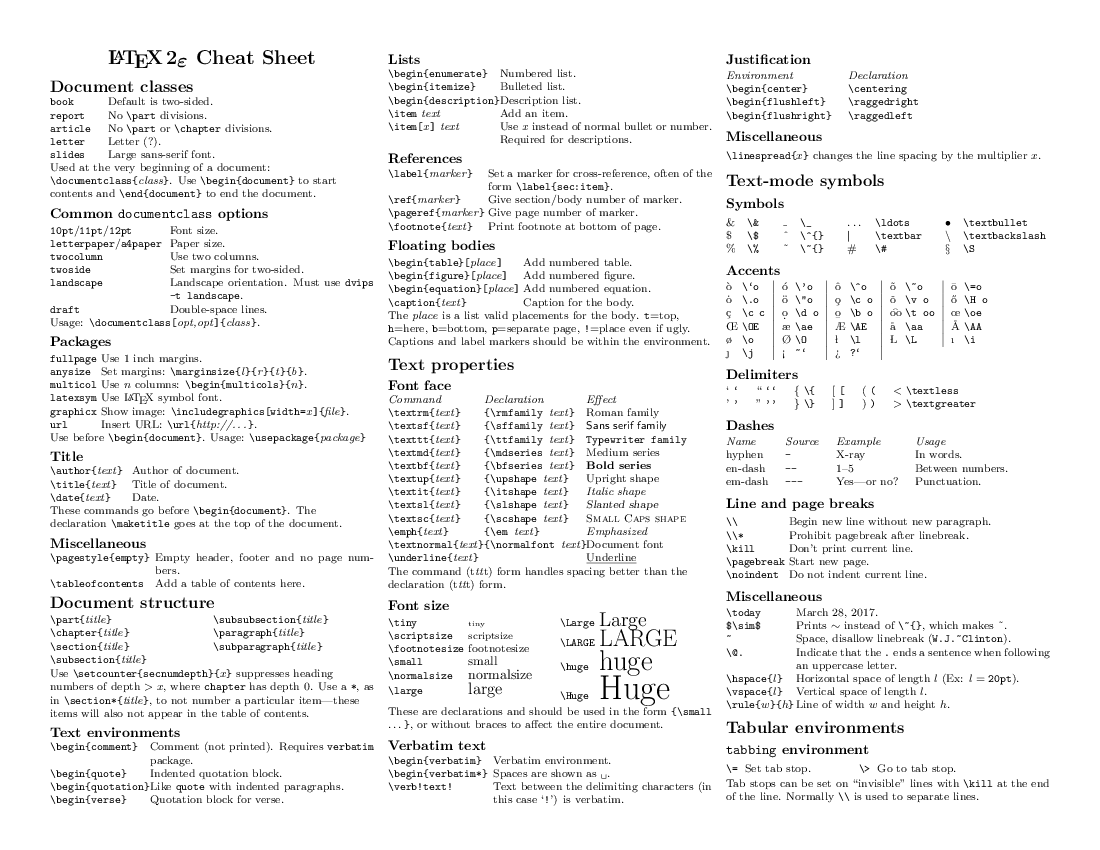
Statistical Distributions
- realpython tutorial on random data
- The Poisson Distribution and Poisson Process Explained
- A Concrete Introduction to Probability (using Python) by Peter Norvig
- wolfram mathworld
- stattrek
- machinelearningmastery - discrete probability distributions
- Online Statistics Education online book
- probability for dummies
- datacamp probability distributions tutorial
- ucd sheet
- 6 common probability distributions blog
Binomial Distribution
Random Numbers
- pythonprogramming
- Khan academy random vs pseudorandom number generators
- machinelearningmaster - random number generators intro
- Analytics Training -random numbers applications
- blog on why randomness matters
Miscellaneous
- Numpy logo. David Cournapeau [BSD], via Wikimedia Commons