- Explain the use and purpose of at least five “Distributions” functions.
Samples of random numbers can be drawn from a variety of probability distributions. The complete list of such functions is listed under Distributions section of the numpy.random reference guide but for the purposes of the assignment I am looking at the following 5 of distribution functions.
Numpy Random Distribution Functions
- The Normal (Gaussian) Distribution Function
- The Standard Normal distribution function
- The Uniform Distribution function
- The Binomial Distribution function
- The Poisson Distribution Function
Each of the numpy.random distribution functions generate different random numbers according to different probabilities over different intervals and can be used to simulate and understand data. There are specific applications and uses for each type of distribution. However the distributions can nearly all be related to each other or transformed into each other in some way or other.
A probability distribution specifies each possible value that a random variable can assume with its probability of occurring. A random variable is any quantity that is assumed to have a probability distribution. Probability is a mathematical expression of uncertainty of the chance of a random variable taking on particular values. There are many different patterns of probability and random numbers can be drawn from various probability distributions.
A discrete random variable is one where its set of possible values is a collection of isolated points on the number line - it has a finite set of specific outcomes, while a continuous random variable is one where its set of possible values is an entire interval on the number line. Discrete random variables almost always come from counting while continuous random variables mostly come from measurement.
Probability distributions are used widely in statistical analysis, data analytics and machine learning. Probability distributions can be simulated based on their mathematical properties. Probability distributions are derived from variance or uncertainty and show which outcomes are more likely and which are less likely.
The probability distribution of a discrete random variable is often known as a probability function or a probability mass function while the probability distribution for a continuous random variable often called a mathematical a probability density function, a frequency function or a probability distribution. Probability distributions can be shown as a formula, a table or a graph.
A Probability Mass Function (PMF) returns the probability of a given outcome while a Cumulative Distribution Function (CDF) returns the probability of a value less than or equal to a given outcome and a Percent-Point Function (PPF) returns a discrete value that is less than or equal to the given probability.
If you can define a probability distribution for a dataset you are interested in, you can use the known properties of the distribution to investigate and summarise the data using statistics, plot the data and look at predicting future outcomes.
If you are interested in measurements of a population but it is not practical to measure this parameter, you could take representative samples from the population and get the average of the samples instead. A statistic is a good estimator for a population parameter and measure estimates of population parameters in a sample.
There are many ways to take samples from a population and when you calculate the average of an individual sample it is unlikely to be the actual true average for the population. You could take samples of a sample size from the population and repeat this process a number of times. NumPy random distribution functions can be used to imitate this process by simulating many many samples of a set sample size from a distribution such as the normal distribution. The mean and standard deviations from the samples can then be used to get the sampling distribution of the mean. While some random samples may have randomly big or randomly small values, overall you could take the average from each of the samples and relate these to the mean of the overall population you took them from.
Some distributions such as the normal and binomial distributions show a central tendancy around a mean value while others such as the uniform distribution do not show any preference for any one value over another and the values can be spread out anywhere in the range. Some distributions start to resemble the normal distribution under certain conditions such as when the number of samples is very large and therefore the normal distribution can be used as an approximation.
Some distributions such as the normal and binomial distributions show a central tendancy around a mean value while others such as the uniform distribution do not show any preference for any one value over another and the values can be spread out anywhere in the range.
According to machinelearningmastery.com
The two types of discrete random variables most commonly used in machine learning are binary and categorical. The most common discrete probability distributions are the Bernoulli and Multinoulli distributions for binary and categorical discrete random variables respectively, and the Binomial and Multinomial distributions that generalize each to multiple independent trials.
- A binary random variable is a discrete random variable where the finite set of outcomes is in {0, 1}.
- A categorical random variable is a discrete random variable where the finite set of outcomes is in {1, 2, …, K}, where K is the total number of unique outcomes.
(wolfram mathworld, stattrek.com and Wikipedia are good sources for information on probability distributions)
There are many plotting functions in Python libraries such as matplotlib.pyplot and seaborn.
Seaborns distplot is a very convenient way to draw a univariate distribution. It draws a histogram and fits a kernel density estimate. A histogram represents the distribution of one-dimensional data by cutting the data into ranges called bins and shows the number of values in each bin which gives a picture of how the values are distributed and the range in which the most common values fall. The kernel density estimate (kde) plots the shape of a distribution. A kde plot encodes the density of observations on one axis with height on the other axis.
The numpy.random distribution functions take various arguments but location for the centre or mean of the distribution, size for the number of samples and scale for the spread or standard deviation are some commonly used arguments.
The numpy.random.normal() function generates random numbers in a bell shaped curve centred around zero. The numbers near the centre of the distribution have a higher chance of being randomly generated while the numbers further away the centre (at zero) have less chance of being randomly generated. The numpy.random.uniform() function generates numbers between a start and finish point where any one number is as likely to occur as any other number. In a uniform distribution, you would expect to see a fairly straight line at the top while the normal distribution is bell shaped.
($\mu$ is the mean, $\sigma$ is the standard deviation which is the square root of the standard deviation, $\sigma^2$.)
Numpy.Random Distribution Functions.
The Normal (Gaussian) Distribution Function
The numpy.random.normal(loc=0.0, scale=1.0, size=None) function is used to draw random samples from a normal (Gaussian) distribution which has a symmetric, bell shaped density curve density curve described by its mean $mu$ and standard deviation $\sigma$.
The normal distribution is considered one of the most important probability distribution for a continuous random variable. It has a symmetric, bell shaped density curve. It is not one distribution but a family of distributions depending on the value of its mean $\mu$ and standard deviation $\sigma$. The normal distributions occurs often in nature. It describes the commonly occurring distribution of samples influenced by a large number of tiny, random disturbances, each with its own unique distribution. All the small influences add up to get a normal distribution.
According to wolfram mathworld
normal distributions have many convenient properties, so random variates with unknown distributions are often assumed to be normal, especially in physics and astronomy. Although this can be a dangerous assumption, it is often a good approximation due to a surprising result known as the central limit theorem. This theorem states that the mean of any set of variates with any distribution having a finite mean and variance tends to the normal distribution. Many common attributes such as test scores, height, etc., follow roughly normal distributions, with few members at the high and low ends and many in the middle.
Any distribution where the mean, median and mode of the distribution coincides is a Normal distribution. Half of the values are to the left of the centre and half to the right.
A normally distributed random variable x can be denoted as follows: x~ $N(\mu,\sigma^2)$ which means that x is normally distributed with a mean of $\mu$ and a variance of $\sigma^2$.
While all values of a normal distribution have a zero probability as it is a continuous distribution, the mean can be thought of as the centre of the distribution or where the values are more likely to be from and its standard deviation shows how likely a value is to be away from the mean value.
The density curve is symmetrical and centered about its mean. The spread is determined by the standard deviation. The data points near the centre of the distribution have a higher chance of being randomly generated while the numbers further away from the centre of the distribution have less chance of being randomly generated. Data close to the mean occur more frequently than data points further away from the mean.
numpy.random.normal distribution function
The numpy.random.normal function generates random number in a bell shaped curve centred around zero but spread out according to the scale parameter. The function depends on two factors, the mean and the standard deviation.
To use the numpy.random.normal function, the loc argument is used to specify the mean or the centre of the distribution, the scale is used to specify the standard deviation of the distribution and the size is the number of random variables to sample. Otherwise the loc or mean defaults to 0 and scale or standard deviation defaults to 1 which is the same as the Standard Normal Distribution. See below.
The mean of the distribution determines the location of the centre of the plot, while the standard deviation determines the height and shape of the graph. A larger standard deviation will result in a shorter and wider curve while a smaller standard deviation results in a tall and narrow curve.
If you supply three arguments, the first is taken to be the mean $\mu$, the second to be the scale or standard deviations $\sigma^2$ and the last to be the number of data points.
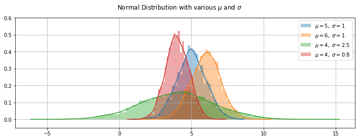
Examples of using the normal distribution function
Below is a plot of 4 normal distribution functions using different values for the loc and scale parameters for the mean and standard deviation of the distribution. This plot shows the distinctive bell shaped curve, which is taller and narrower for the distribution with the smaller standard deviation or spread and wider and flatter for the distribution with the larger standard deviation as the scale parameter. In each case the curve is centred around the mean of the distribution as the loc parameter.
Plotting the Normal Distribution function
Comparing the distribution of two normally distributed variables with different means and standard deviations.
Plotting normal distributions with various means and spreads.
Here I plot different normal distributions with various means and standard deviations.
np.random.normal # <function RandomState.normal>
<function RandomState.normal>
# Generate some random datasets using random.normal
loc,scale,size = 5,1,3000

sample1 = np.random.normal(loc,scale,size)
sample2 = np.random.normal(loc+1, scale,size)
sample3 = np.random.normal(loc-1,scale+1.5,size)
sample4 = np.random.normal(loc-1,scale-0.2, 3000)

# set up the plot figure
plt.figure(figsize=(12,4))  # set the size of the figure
# using seaborn distplot functions to plot given loc(mean) and scale(standard deviation)
sns.distplot(sample1,label="$\mu=5,\ \sigma=1$")
sns.distplot(sample2, label ="$\mu=6,\ \sigma=1$")
sns.distplot(sample3, label="$\mu=4,\ \sigma=2.5$")
sns.distplot(sample4, label ="$\mu=4,\ \sigma=0.8$")
plt.legend(loc="best")
plt.ylim([-0.05, 0.6]) # set the plot limits on the y-axis
plt.suptitle('Normal Distribution with various $\mu$ and $\sigma$')
plt.grid(True)
Verifying the mean and the standard deviation.
The mean is an estimator of the centre of the distribution. The median is another estimator for the centre of the distribution. It is the value where half of the observatins are below and half are above it. The median is not sensitive to the tails of the distribution and is considered robust.
print('The means of the distributions are \n sample1: %.3f, sample2: %.3f, sample3: %.3f and sample 4:%.3f' % (np.mean(sample1), np.mean(sample2),np.mean(sample3),np.mean(sample4)))
print('The medians of the distributions are \n sample1: %.3f, sample2: %.3f, sample3: %.3f and sample 4:%.3f' % (np.median(sample1), np.median(sample2),np.median(sample3),np.median(sample4)))
print('The standard deviations of the distributions are \n sample1: %.3f, sample2: %.3f, sample3: %.3f and sample 4:%.3f' % (np.std(sample1), np.std(sample2),np.std(sample3),np.std(sample4)))
The means of the distributions are
 sample1: 5.010, sample2: 6.000, sample3: 4.049 and sample 4:4.026
The medians of the distributions are
 sample1: 4.999, sample2: 6.029, sample3: 4.077 and sample 4:4.003
The standard deviations of the distributions are
 sample1: 0.990, sample2: 1.007, sample3: 2.510 and sample 4:0.787
The plots above demonstrate the bell-shaped nature of the distributions. Changing the loc parameter for the mean will move the curve along the x-axis while changing the scale parameter result in wider or narrower curves.
There is a general rule that 68.27% of the values under the curve fall between -1 and +1 standard deviations from the mean or centre, 95.45% under the curve between -2 and 2 standard deviations and 99.73% between -3 and 3 standard deviations. This rule applies no matter what the mean and standard deviations are. For any normally distributed variable, irrespective of it’s mean and standard deviation, if you start at the mean and move one standard deviation out in any direction, the probability of getting a measurement of value from this variable within this range is just over 68%, the probability of getting a value within two standard deviations is over 95% and the probability of getting a value within 3 standard deviations from the mean is 99.73%. This leaves a very small percentage of values that lie further than 3 standard deviations from the mean.
The curves do not not actually cross the x-axis at all as it goes to infinity in both directions of the mean. However the chances of observing values more than 3 standard deviations from the centre or mean of the curve is very small.
All the plots above are normally distributed but with different means $\mu$ and standard deviations $\sigma$. A normal distribution with a mean of 0 and a standard deviation of 1 is a special case of the normal distribution which brings me to the next distribution - the Standard Normal Distribution.
The Standard Normal Distribution function
For an approximately normal data set, almost 68% of the data points fall within one standard deviation from the mean, while 95% of the data falls within 2 standard deviations and 99.7% fall within 3 standard deviations.
There are many different normal distributions with different means and variances which would have made them difficult to have been tabulated in the statistical tables. The standard normal distribution is a special case of the normal distribution with $\mu$ of 0 and standard deviation $\sigma$ of 1 and this is tabulated and can be used to find the probabilities for any normal distribution. All questions regarding the normal distribution can be converted into questions regarding the standard normal distribution.
The standard normal distribution is a special case of the normal distribution.
It is the distribution that occurs when a normal random variable has a mean of zero and a standard deviation of one. The normal random variable of a standard normal distribution is called a standard score or a z score. Every normal random variable X can be transformed into a z score.
The numpy.random.standard_normal distribution function is used to draw samples from a Standard Normal distribution that has a mean of 0 and a standard deviation of 1. The standard normal distribution, of the random variable z, has $\mu$ = 0 and $/sigma$ = 1 and can be used to calculate areas under any normal distribution. z~ $N(0,1)$
To use this numpy.random.standard_normal function, you just need to supply the number of data points to generate as the size argument. Without specifying the number of data points you will just get a single value.
Note that the numpy.random.randn() function in the section on simple random data functions a convenience function for numpy.random.standard_normal. It returns a single float or an ndarray of floats. See numpy.random.randn.
np.random.standard_normal # <function RandomState.standard_normal>
<function RandomState.standard_normal>
# Generate some random samples from standard normal distributions

sample1 = np.random.standard_normal(100) # only need to set the size of the samples
sample2 = np.random.standard_normal(500)
sample3 = np.random.standard_normal(1000)
sample4 = np.random.standard_normal(2000)
# set up the plot figure size

plt.figure(figsize=(12,4))
# using seaborn kdeplot functions to plot
sns.kdeplot(sample1,shade=True,label="size=100")
sns.kdeplot(sample2, shade=True,label ="size=500")
sns.kdeplot(sample3, shade=True,label ="size=1000")
sns.kdeplot(sample4, shade=True,label ="size=2000")

plt.legend(loc="best") # set the legends
plt.suptitle('The Standard Normal Distribution with various $\mu$ and $\sigma$') # the title of the plot
plt.grid(True)
plt.ylim([-0.05, 0.5]) # set the plot limits on the y-axis
print('The means of the distributions are \n sample1: %.3f, sample2: %.3f, sample3: %.3f and sample 4:%.3f' % (np.mean(sample1), np.mean(sample2),np.mean(sample3),np.mean(sample4)))
print('The medians of the distributions are \n sample1: %.3f, sample2: %.3f, sample3: %.3f and sample 4:%.3f' % (np.median(sample1), np.median(sample2),np.median(sample3),np.median(sample4)))
print('The standard deviations of the distributions are \n sample1: %.3f, sample2: %.3f, sample3: %.3f and sample 4:%.3f' % (np.std(sample1), np.std(sample2),np.std(sample3),np.std(sample4)))
print("\n")
The means of the distributions are
 sample1: -0.180, sample2: 0.016, sample3: -0.032 and sample 4:-0.029
The medians of the distributions are
 sample1: -0.183, sample2: -0.007, sample3: -0.040 and sample 4:-0.024
The standard deviations of the distributions are
 sample1: 0.976, sample2: 0.964, sample3: 0.951 and sample 4:1.034
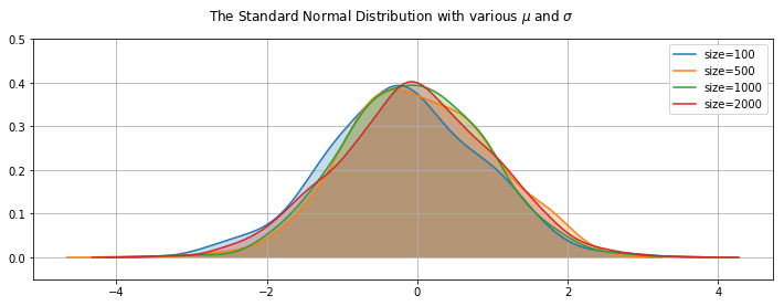
The above plots show that whatever the number of values generated, the curve is always centred about the mean of 0, most of the values are clustered around the centre and most of the values are within 2 standard deviations of the mean. As the size of the sample increases, the shape becomes more symetrical.
The Uniform distribution functions.
The continuous Uniform distribution function is one of the simplest probability distributions where all it’s possible outcomes are equally likely to occur. It has constant or uniform probability.
Wikipedia describes the Uniform Distribution as the continuous uniform distribution or rectangular distribution is a family of symmetric probability distributions such that for each member of the family, all intervals of the same length on the distribution’s support are equally probable. The support is defined by the two parameters, a and b, which are its minimum and maximum values.
The continuous uniform distribution takes values in the specified range (a,b). The curve describing the distribution is rectangle shaped because any interval of numbers has the same probability of being drawn as any other interval of the same width. Each interval has constant height across it and 0 everywhere else. The area under the curve must be equal to 1 and therefore the height of the curve equals $\frac{1}{b-a}$. The probability density function of a uniformly distributed variable x is $f(x)= \frac{1}{a-b}$ if $a<=x<=b$ or zero otherwise.
The expected value of the uniform distribution is $\frac{b+a}{2}$ the midpoint of the interval and the variance $\sigma^2$ is $\frac{1}{12}(b-a)^2$.
When the interval is between 0 and 1, it is known as the Standard Uniform distribution. The Standard Uniform distribution, where a is 0 and b is 1 is very commonly used for random number generation and in statistics in general. The expected value of the standard uniform distribution is $\frac{1}{2}$ and the variance is $\frac{1}{12}$.
As all outcomes are equally likely there is no one particular value that occurs more frequently than any other and therefore there is no skew in a uniform distribution like there is in other distributions.
The uniform distribution can be used to generate random numbers between a minimum and a maximum value where each number is equally likely to occur. Rolling a dice several times is an example of the uniform distribution, where each number on the dice is equally likely to occur on each roll. No single side of the dice has a higher chance than another.
While many natural things in the world have approximately normal distributions where values are more likely to fall in the centre of the distribution, a uniform distribution can be used for modeling events that are equally likely to happen in a given interval between a minimum and a maximum range. This minimum value is usually referred to as a while the maximum value is referred to as b.
If a random variable is uniformly distributed between a minimum (a) and maximum value (b), then the distribution can be used to calculate the probability that a value will lie in a cetain part of the interval, say between two points c and d where d > c. The probability for something in such an interval is calculated using $\frac{d-c}{b-a}$.
The numpy.random.uniform function.
numpy.random.uniform(low=0.0, high=1.0, size=None
Samples are uniformly distributed over the half-open interval $[low, high)$ (includes low, but excludes high). In other words, any value within the given interval is equally likely to be drawn by uniform.
To use this function, you provide the lower $low$ and upper $high$ bounds of the interval to specify the minimum (a) and maximum (b) possible values in the range. The smaller number provided will be taken as the lower bounds and the bigger number as the upper bound. Without providing an interval bounds, the function assumes a standard uniform distribution.
The function randomly samples from the uniform distribution over the specified interval. If not argument at all is provided then it will return a single value in the interval $[0.0,1.0)$. If a single value is provided to the function, a single value will be returned from the interval between 0 and that number. If two values are provided, then a single value will be returned from the interval between between these two numbers. A third value provided will be used as the size of the array returned.
The simple numpy.random.rand function in section 2 also returns samples from the continuous uniform distribution but only in the $[0.0, 1.0)$ interval. The other numpy.random functions random_sample,random, sample and ranf can be used to sample from $[a,b)$ intervals other than between 0 and 1 by multiplying the output by $(b-a)$ and adding $a$ but the numpy.random.uniform function is easier to use for this purpose.
Sampling from the continuous uniform distribution
The following are examples of using the numpy.random.uniform function where various numbers of arguments are provided as outlined above.
np.random.uniform() # returns a single random value in the interval [0,1)
np.random.uniform(5) # returns a single value from the interval $[0,5)$
np.random.uniform(5,10) # returns a single value in the interval [6,10)]
np.random.uniform(5,10,15) # returns an array of 15 values from the interval [5,10)
Here I show that the mean and median values are very close, while the mean is the midpoint of the interval and the variance is equal to $\frac{1}{12}(b-a)^2$. If the size of the sample is changed in the code below, the mean and median get closer and closer to each other and to the expected value. These results are the same no matter what interval $[a,b)$ is used. Also showing that all the values are from the interval $[a,b)$
np.random.uniform #<function RandomState.uniform>
<function RandomState.uniform>
a,b,size = 5,10,500

x = np.random.uniform(a,b,size) # returns an array of 500 values from the interval [5,10)
print(x)
print('\n Expected value is %.3f, Variance: %.3f' % ((b+a)/2, ((b-a)**2)/12))
print('The mean is %.3f, the median is %.3f' % (np.mean(x), np.median(x)))

# Checking that all the values are within the given interval:
print(np.all(x >= a))

print(np.all(x < b))
[6.4056 8.1328 9.8728 ... 7.08   5.946  7.4204]

 Expected value is 7.500, Variance: 2.083
The mean is 7.465, the median is 7.439
True
True
Using the same random.seed to show the similarity between the numpy.random.uniform is similar to numpy.random.random
# 100 values from the uniform 2,11] interval
np.random.seed(1)
u1 = np.random.uniform(2,11,100)
np.random.seed(1)
u2 =(b-a)* np.random.random((100)) +a
u1 ==u2
array([False, False, False, ..., False, False, False])
Plotting Uniform distributions
# generate random sample of 1000 from two different intervals
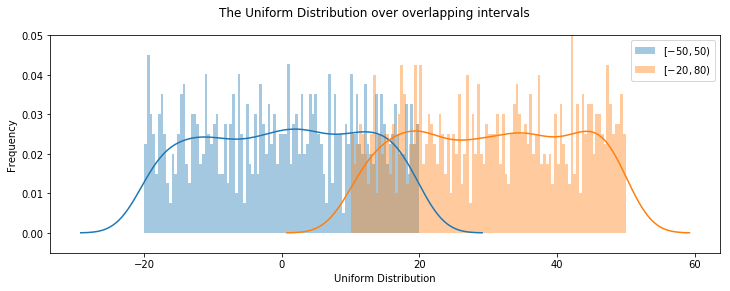
a,b, size = -20,20,1000 # set the a,b and size parameters
u1 = np.random.uniform(a,b,size) # sample from -20,20 interval
u2 = np.random.uniform(a+30, b+30, size)# sample from -10,50 interval
plt.figure(figsize=(12,4)) # set up the figure size for the plot
ax = sns.distplot(u1, bins=100, label="$[-50,50)$"); # distplot using 100 bins
ax = sns.distplot(u2, bins=100, label="$[-20,80)$");
ax.set(xlabel="Uniform Distribution", ylabel ="Frequency") # set the x-axis and y-axis labels
plt.legend() #
plt.suptitle("The Uniform Distribution over overlapping intervals")
plt.ylim([-0.005,0.05])
print('The mean of u1 is %.3f' % np.mean(u1)) # to 3 decimal places
print('The mean of u2 is %.3f' % np.mean(u2)) # to 3 decimal places
The mean of u1 is 0.115
The mean of u2 is 30.516
Plotting samples of size 1000 from continuous uniform distributions across various interval using matplotlib plots
Also showing the means which can be seen as the midpoint of the intervals for each distribution.
Using the example then from themanual to plot a histogram of a uniform distribution function and its probability density function using the np.ones_like function. The area under the curve between a and b is 1
# create samples from uniform distribution over different intervals but the same size
x1 = np.random.uniform(2,12,1000)
x2 = np.random.uniform(5,20,1000)
x3 = np.random.uniform(2,20,1000)
x4 = np.random.uniform(-5,5,1000)

plt.figure(figsize=(12, 3)) # set up the figure
plt.subplot(141) # select 1st of 4 plots
plt.hist(x1) # plot first sample x1
plt.subplot(142) # select 2nd of 4 plots
plt.hist(x2) # plot second sample x2
plt.subplot(143)
plt.hist(x3)
plt.subplot(144)
plt.hist(x4)
plt.suptitle('Uniform Distribution over various intervals')
plt.show()
print('The means of these distributions are for x1: %.3f, x2: %.3f, x3: %.3f and x4: %.3f' %(np.mean(x1), np.mean(x2), np.mean(x3), np.mean(x4))) # to 3 decimal places
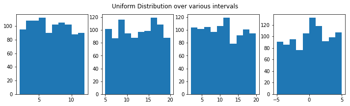
The means of these distributions are for x1: 6.897, x2: 12.541, x3: 10.816 and x4: 0.178
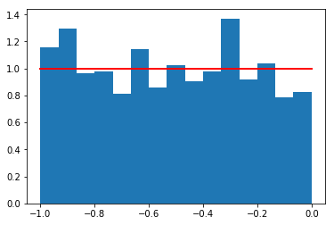
# Example from the numpy.random.uniform reference manual
#Display the histogram of the samples, along with the probability density function:
s = np.random.uniform(-1,0,1000)
# use np.ones_like function to return an array of ones with the same shape and type as s.
import matplotlib.pyplot as plt

count, bins, ignored = plt.hist(s, 15, density=True) # use 15 bins
plt.plot(bins, np.ones_like(bins), linewidth=2, color='r') ## add a horizontal line at 1.0 using the np.ones like
plt.show()
The Binomial Distribution
The numpy.random.binomial function is used to draw samples from a Binomial Distribution which is considered one of the most important probability distributions for discrete random variables. The Binomial distribution is the probability distribution of a sequence of experiments where each experiment produces a binary outcome and where each of the outcomes is independent of all the others.
The binomial distribution is the probability of a success or failure outcome in an experiment that is repeated many times. A binomial experiment has only two (bi) possible outcomes such as heads or tails, true or false, win or lose, class a or class b etc. One of these outcomes can be called a success and the other a failure. The probability of success is the same on every trial A single coin flip is an example of an experiment with a binary outcome.
According to mathworld.wolfram, the Binomial Distribution gives the discrete probability distribution $P_p(n|N)$ of obtaining exactly n successes out of N Bernoulli trials (where the result of each Bernoulli trial is true with probability $p$ and false with probability $q=1-p$). See also https://en.wikipedia.org/wiki/Binomial_distribution.
The results from performing the same set of experiments, such as repeatedly flipping a coin a number of times and the number of heads observed across all the sets of experiments follows the binomial distribution.
$n$ is usually used to denote the number of times the experiment is run while $p$ is used to denote the probability of a specific outcome such as heads.
A Bernoulli trial is a random experiment with exactly two possible outcomes, success and failure, where probability of success is the same every time the experiment is conducted. A Bernoulli process is the repetition of multiple independent Bernoulli trials and it’s outcomes follow a Binomial distribution. The Bernoulli distribution can be considered as a Binomial distribution with a single trial (n=1).
A binomial experiment consists of a number $n$ of repeated identical Bernoulli trials
- where there are only two possible outcomes, success or failure
- the probability of success $p$ is constant (the same in every trial)
- the $n$ trials are independent - outcome of one trial does not affect the outcome of another trial.
- The binomial random variable $x$ is the number of successes in $n$ trials.
The outcome of a binomial experiment is a binomial random variable. Binomial probability is the probability that a binomial random variable assumes a specific value. -b(x,n,P): Binomial probability - the probability that an n-trial binomial experiment results in exactly x successes.
The binomial distribution has the following properties:
- The mean of the distribution is equal to $n*P$
- The variance $\sigma^2$ is $nP(1-p)$
- the standard deviation $sqrt(nP(1-p))$
Some other properties of the Binomial Distribution from Wikipedia:
- In general, if
npis an integer, then the mean, median, and mode coincide and equalnp. - The Bernoulli distribution is a special case of the binomial distribution, where n = 1.
- The binomial distribution is a special case of the Poisson binomial distribution, or general binomial distribution, which is the distribution of a sum of n independent non-identical Bernoulli trials B(pi)
- If n is large enough, then the skew of the distribution is not too great. In this case a reasonable approximation to B(n, p) is given by the normal distribution
- The binomial distribution converges towards the Poisson distribution as the number of trials goes to infinity while the product np remains fixed or at least p tends to zero. Therefore, the Poisson distribution with parameter λ = np can be used as an approximation to B(n, p) of the binomial distribution if n is sufficiently large and p is sufficiently small. According to two rules of thumb, this approximation is good if n ≥ 20 and p ≤ 0.05, or if n ≥ 100 and np ≤ 10.[
Using the numpy.random.binomial function
The numpy.random.binomial function is used to sample from a binomial distribution given the number of trials $n$ and the probability $p$ of success on each trail. The number of samples $size$ represents the number of times to repeat the $n$ trials.
This function takes an integer to set the number of trials which must be greater than or equal to zero. The probability must be in the interval $0,1]$ as total probability always sums to one. It returns an array of samples drawn from the binomial distribution based on the $n$ and $p$ and $size$ parameters given to the function. Each sample returned is equal to the number of successes over n trials.
The np.random.binomial(n, p) function can be used to simulate the result of a single sequence of n experiments (where n could be any positive integer), do so using using a binomially distributed random variable.
For example to find the probability of getting 4 heads with 10 coin flips, simulate 10,000 runs where each run has 10 coin flips. This repeats the 10 coin toss 10,000 times.
Example of drawing samples from a binomial distribution.
Draw samples from a distribution using np.random.binomial(n, p, size) where:
- $n$ the number of trials,
- $p$ the probability of success in each trial
- $size$ is the number of samples drawn (the number of times the experiment is run)
np.random.binomial # <function RandomState.binomial>
<function RandomState.binomial>
n, p = 10, .5  # number of trials, probability of each trial
s = np.random.binomial(n, p, 100)
print(s)  ## returns an array of 100 samples
print(np.size(s))
[2 8 5 ... 4 5 8]
100
This returns a numpy array with 100 (size=100) samples drawn from a binomial distribution where the probability of success in each trial is 0.5 (p=0.5), where each number or sample returned represents the number of successes in each experiment which consist of 10 bernoulli trials (n=10)
These 100 number represents the number of successes in each experiment where each experiment consists of 10 bernoulli trials each with 0.5 probability of success.
[ 8 10 2 ... 6 5 5]
8 out of 10 successes in the first experiment of 10 trials, 10 successes in the second experiment of 10 trials, 2 out of 10 successes in the third experiment of 10 trials etc..
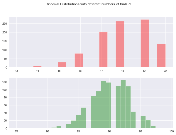
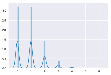
Plotting the Binomial distribution
Here I am using seaborn to plot a Binomial distribution that has 100 trials in each experiment, the probability of success in each trial is 0.9 and the number of samples (or times the experiment is run) is 1000. As the plot shows, the distribution is skewed to the right because the probability of success in each trial is 0.9 so more samples will have more successes. When the probability of success is less than 0.5 then a left skewed distribution is expected. The probability of success probability determines the skew. A probability of 0.5 would have a centred distribution.
If n is large enough, then the skew of the distribution is not as great and as mentioned above, a reasonable approximation to B(n, p) is given by the normal distribution.). When I increase the number of trials by multiples while keeping the same probability the skew becomes lesser and the curve looks more ‘normal’.
sns.set_style('darkgrid')
n,p,size = 20, 0.9, 1000 # # number of trials, probability of success in each trial, number of samples (experiments run)
# Generate a random datasets using random.binomial
np.random.seed(10)
b11 = np.random.binomial(n, p, size) # p= 0.1
b22 = np.random.binomial(n*5, p, size) # p= 0.3

# Set up the matplotlib figure
f,axes = plt.subplots(2,1,figsize=(10,7),sharex=False)

sns.distplot(b11, label="p=0.1", kde=False,color="r",ax=axes[0]) # p=0.1
sns.distplot(b22, label="p=0.3", kde=False, color="g",ax=axes[1]) # p=0.5
plt.suptitle("Binomial Distributions with different numbers of trials $n$")

plt.show()
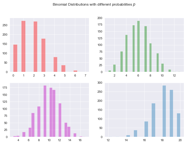
Plotting the binomial distribution with various probabilities.
Below I plot binomial distribution with increasing probabilities. The bottom left curve with probabilites of 0.5 is centred while the sample with lower probability is right skewed and the samples with probabilites closer to 1 are left skewed.
# Set up the matplotlib figure

sns.set_style('darkgrid')
n,p,size = 20, 0.1, 1000 # # number of trials, probability of success in each trial, number of samples (experiments run)
# Generate a random datasets using random.binomial

b1 = np.random.binomial(n, p, size) # p= 0.1
b2 = np.random.binomial(n, p+0.2, size) # p= 0.3
b3= np.random.binomial(n, p+0.4, size) # p= 0.5
b4= np.random.binomial(n, p+0.8, size) # p= 0.9

# Set up the matplotlib figure
f,axes = plt.subplots(2,2,figsize=(10,7),sharex=False)

sns.distplot(b1, label="p=0.1", kde=False, color="r",ax=axes[0,0]) # p=0.1
sns.distplot(b2, label="p=0.3", kde=False, color="g",ax=axes[0,1]) # p=0.5
sns.distplot(b3 ,label="p=0.5", kde=False, color="m",ax=axes[1,0]) # p=0.9
sns.distplot(b4 ,label="p=0.9", kde=False, ax=axes[1,1]) # p=0.9


plt.suptitle("Binomial Distributions with different probabilities $p$")
ax.set(xlabel="Binomial Distribution", ylabel ="Frequency")

plt.show()
print('The means of these distributions are for b1: %.3f, b2: %.3f, b3: %.3f and b4: %.3f' %(np.mean(b1), np.mean(b2), np.mean(b3), np.mean(b4))) # to 3 decim
looking at the statistics: mean, median, mode, variance and standard deviation
Here I check that the mean of the distribution is equal to $nP$ and that the standard deviation is equal to $sqrt(nP*(1-p))$. In general, if np is an integer, then the mean, median, and mode coincide and equal np. This is shown below where the mean, median and mode are very similar and equal to n times p.
There seems to be no mode function in numpy but there is one in the scipy.stats package which I use here.
n,p,size = 30, 0.3, 10000 # # number of trials, probability of success in each trial, number of samples (experiments run)
# Generate a random datasets using random.binomial

s1 = np.random.binomial(n, p, size) # p= 0.3

from scipy import stats # no mode in numpy
print('Mean: %.3f'% np.mean(s1), 'Median: %.3f' % np.median(s1),'Standard Deviation: %.3f' % np.std(s1))

print('n times p : %.3f'% (n*p))
print('np.sqrt(n*p*(1-p)) %.3f' %np.sqrt(n*p*(1-p)))
stats.mode(s1)
Mean: 8.970 Median: 9.000 Standard Deviation: 2.533
n times p : 9.000
np.sqrt(n*p*(1-p)) 2.510


ModeResult(mode=array([9]), count=array([1625]))
Example of using numpy.random.binomial
The numpy random reference docs demonstrates the following real world example.
A company drills 9 wild-cat oil exploration wells, each with an estimated probability of success of 0.1. All nine wells fail. What is the probability of that happening? To do this, 20,000 trials of the model are simulated and then the number generating zero positive results are counted where n = 9, p = 0.1 and size = 20,000
Below I use the example and expand on it:
# set the parameters and create a sample, then check how many trials resulted in zero wells succeeding
n,p,size = 9, 0.1, 20000
s =np.random.binomial(n, p, size)
print(sum(s == 0)/20000.) # what is probability of all 9 wells failing.
0.388
This shows that there is a 39% probability of all 9 wells failing (0 succeeding) but I could also check the probability of all 9 being successful which is 0. The distribution plot shows the probabilities for each possible outcome. Below I use a lambda function to check for the probability for 0,1,2 .. up to all the 9 wells being successful. This corresponds with the plot below which shows that no well succeeding or only 1 well succeeding have the highest probabilites. The probabilites of more than two wells succeeding given p=0.1 is very small and the probabilities of more than two successful wells is very very small.
print(sum(s == 0)/20000.) # what is probability of all 9 wells failing.
print(sum(s == 9)/20000.) # probability of all 9 successeding
print(sum(s == 1)/20000.) #probability of 1 well being successful
0.388
0.0
0.38415
Write a lambda function to check the probabilties of 0,1,2,3.. up to all 9 wells failing.
n,p,size = 9, 0.1, 20000 ## set the probability of success, number of bernouilli trials and number of samples or experiments
g = lambda x: sum(np.random.binomial(n,p,size)==x)/size #

[g(i) for i in range(10)] ## run the lambda function g to get the probabilities for the numbers in the range 0 to 9
[np.mean(g(i)) for i in range(10)] # get the average
[0.3932, 0.3885, 0.17705, 0.04515, 0.00685, 0.00075, 0.0001, 0.0, 0.0, 0.0]
sns.distplot(s)
<matplotlib.axes._subplots.AxesSubplot at 0x1a1daeefd0>
If the probabiility is p=0.3 with n=10 trials in each experiment then the expected number of successful outcomes is 3 out of 10 trials in each experiment.
The Binomial distribution summarizes the number of successes k in a given number of Bernoulli trials n, with a given probability of success for each trial p.
The examples on machinelearningmastery show how to simulate the Bernoulli process with randomly generated cases and count the number of successes over the given number of trials using the binomial() NumPy function. However these examples also make use of the scipy-stats-binom function but I will use these as a basis for an example using numpy.random.binomial function.
This numpy.random.binomial function takes the total number of trials and probability of success as arguments and returns the number of successful outcomes across the trials for one simulation.
- With n of 100 and p of 0.3 we would expect 30 cases to be successful.
- Can calculate the expected value (mean) and variance of this distribution.
n,p,size = 100, 0.3, 1000 ## set the probability of success, number of bernouilli trials and number of samples or experiments
s3 = np.random.binomial(100, 0.3, 1000)
plt.figure(figsize=(10,4))
sns.distplot(s3)
print(np.mean(s3))
30.133
# example of simulating a binomial process and counting success
import numpy as np
# define the parameters of the distribution
n,p = 100, 0.3
# run a single simulation
success = np.random.binomial(n, p)
print('Total Success: %d' % success)
Total Success: 26
# 2
print('Mean=%.3f, Variance=%.3f' % (np.mean(success), np.var(success)))
Calculate the probaility of so many successes in every 100 trials. Do this in steps of 10. This shows that as expected, 30 successful outcomes has the highest probability.
n,p,size = 100, 0.3, 10000 ## set the probability of success, number of bernouilli trials and number of samples or experiments
g = lambda x: sum(np.random.binomial(n,p,size)==x)/size*100 #
[g(i) for i in range(10,110,10)] ## run the lambda function g to get the probabilities for the numbers in the range 0 to 9
n,p=100,0.3

for x in range(10,110,10):  # go up in steps of 10
    success =np.random.binomial(n, p) ## calculate the number of successes
    print('probability of ',x,'successes in ',n, 'trials is', sum(np.random.binomial(n,p,size)==x)/100,'%')
The Poisson Distribution function
The numpy.random.poisson function is used to draw samples from a Poisson distribution. It takes a $\lambda$ parameter as well as a size for the number of samples.
numpy.random.poisson(lam=1.0, size=None)
The Poisson distribution is the limit of the binomial distribution for large N.
The Poisson distribution, named after French mathematician Siméon Denis Poisson, is a discrete probability distribution that expresses the probability of a given number of events occurring in a fixed interval of time or space if these events occur with a known constant rate and independently of the time since the last event. The Poisson distribution can also be used for the number of events in other specified intervals such as distance, area or volume.
It was originally developed in France in the 1830’s to look at the pattern of wrongful convictions in a year. A poisson distribution gives the probability of a number of events in an interval generated by a Poisson process which is a model for describing randomly occuring events. It is defined by the rate parameter, $\lambda$, which is the expected number of events in the interval.
A poisson random variable can be used to model the number of times an event happened in a time interval. A poisson distribution is the probability distribution of independent occurences of an event in an interval. It can be used for finding the probability of a number of events in a time period, or the probability of waiting some time until the next event occurs. When you know how often an event has occurred then you can it to predict the probability of such events happening.
The poisson probability distribution function takes one parameter which is lamda $\lambda$ or the rate parameter which is a function of both the average events per time and the length of the time period or the expected number of events in an interval. It can be used for count based distributions where the events happen with a known average rate and independently of time since the last event such as the number of times an event occurs in an interval of time or space such as number of winning lottery tickets per week, the number of visitors to a website in a period, the number of patients admitted to a hospital A&E in a particular hour, the number of goals scored by a team in a match etc.
An event can occur 0, 1, 2, … times in an interval. The average number of events in an interval is designated $\lambda$ which is the event rate known as the rate parameter. To find the probability of observing $k$ events in an interval you use the following formula:
$${\displaystyle P(k{\text{ events in interval}})={\frac {\lambda ^{k}e^{-\lambda }}{k!}}}$$
where $\lambda$ is the average number of events per interval, $e$ is the number 2.71828 (which is the base of the natural logarithms), $k$ takes values 0, 1, 2, … $k! = k * (k − 1) * (k − 2) * … * 2 * 1 $is the factorial of k.
As the rate parameter $\lambda$ is changed, the probability of seeing different numbers of events in one interval is changed. The most likely number of events in the interval for each curve is the rate parameter which is the only number needed to define the Poisson distribution. (As it is a product of events/interval and the interval length it can be changed by adjusting the number of events per interval or by adjusting the interval length).
If you give the numpy.random.poisson function the mean or average number of occurances as $\lambda$, it returns the probability that $k$ number of events will occur.
The default settings is $\lambda$ = 1 and generate a single value.
(lam=1.0, size=None)
If you supply a rate parameter of 5 to the numpy.random.poisson function it will randomly generates numbers from 0,1,2,3 up to infinity but the most likely number to occur will be 5, followed by the numbers closer to 5 such as 3 and 4.
You can also specify how many samples to generate if you want more than a single number.
Using the numpy.random.poisson function.
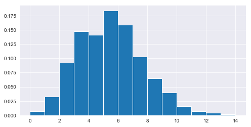
Starting off with the example from the documentation, set $\lambda$ to 1 and draw 1000 values from a poisson distribution that has a rate of 5.
np.random.poisson # <function RandomState.poisson>
import numpy as np  # from documentation
plt.figure(figsize=(8,4)) # set the figure size
s = np.random.poisson(5, 1000) # lambda 5, 1000 samples
import matplotlib.pyplot as plt
count, bins, ignored = plt.hist(s, 14, density=True) # plot histogram of values
plt.show()
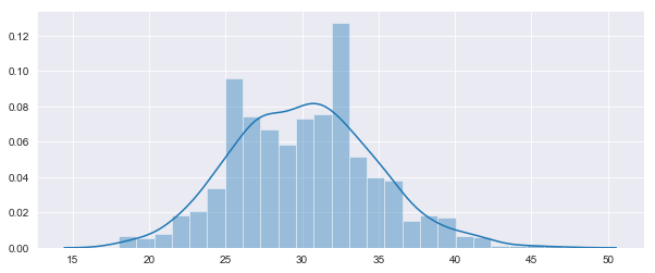
Draw values from poisson distributions with different $\lambda$ values
Here I will draw samples from poisson distributions with different rate parameters in a 10 by 5 array. Create a DataFrame and then look at the summary statistics using the pandas.describe function. The expected value, variance and lambda should all be very close.
# Draw each 10 values for lambda 5,10,15,20 and 50
s = np.random.poisson(lam=(5, 10,15,20,50), size=(1000, 5))
import pandas as pd
poissondf= pd.DataFrame(s, columns=['lambda=5','lambda10','lambda=15','lambda=20','lambda=50'])
print(poissondf.describe())
print("\n Variances")
print(poissondf.var())
          lambda=5     lambda10   lambda=15    lambda=20    lambda=50
count  1000.000000  1000.000000  1000.00000  1000.000000  1000.000000
mean      4.975000    10.002000    14.84000    19.857000    49.690000
std       2.217948     3.154988     3.75453     4.407037     7.100586
min       0.000000     2.000000     5.00000     8.000000    30.000000
25%       3.000000     8.000000    12.00000    17.000000    45.000000
50%       5.000000    10.000000    15.00000    20.000000    49.000000
75%       6.000000    12.000000    17.00000    23.000000    54.000000
max      13.000000    22.000000    29.00000    34.000000    72.000000

 Variances
lambda=5      4.919294
lambda10      9.953950
lambda=15    14.096496
lambda=20    19.421973
lambda=50    50.418318
dtype: float64
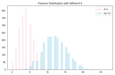
Again drawing samples from another poisson distribution with different $\lambda$’s
The curves show the peak around the expected value equal to $\lambda$. The curve shifts depending on the mean.
# Set up the matplotlib figure

plt.figure(figsize=(8,5))
sns.set_style('white')
lam,size = 4,2000
# Generate a random datasets using random.binomial
p1 = np.random.poisson(lam, size)
p2 = np.random.poisson(lam+8, size)

sns.distplot(p1,label = "$\lambda$=4", kde=False,color="pink") #
sns.distplot(p2, label = "$\lambda$a=12", kde=False, color="skyblue") #

plt.legend()
plt.title("Poisson Distribution with different $\lambda$")
plt.show()
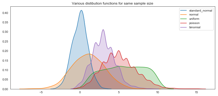
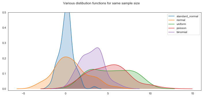
Showing the various distributions
size =100
sn1 = np.random.standard_normal(size)
n1 = np.random.normal(1,2,size)
u1 = np.random.uniform(1,10,size)

p1 = np.random.poisson(5, size)
b1 = np.random.binomial(10, 0.3, size)
plt.figure(figsize=(12,5)) # set up the figure size

# plotting the various distributions using kde plot, setting legends
sns.kdeplot(sn1, label ="standard_normal", shade=True) # using the kde plots and shading in
sns.kdeplot(n1, label ="normal", shade=True)
sns.kdeplot(u1, label = "uniform", shade=True)
sns.kdeplot(p1, label = "poisson", shade=True)
sns.kdeplot(b1, label = "binomial",shade=True)
plt.suptitle("Various distibution functions for same sample size")
plt.ylim([-0.01,0.5]) # set the y axis
plt.legend() # show the legends
plt.show()
size =1000
sn2 = np.random.standard_normal(size)
n2 = np.random.normal(1,2,size)
u2 = np.random.uniform(1,10,size)
p2 = np.random.poisson(5, size)
b2 = np.random.binomial(10, 0.3, size)
plt.figure(figsize=(12,5))
sns.kdeplot(sn2, label ="standard_normal",shade=True)
sns.kdeplot(n2, label ="normal",shade=True)
sns.kdeplot(u2, label = "uniform",shade=True)
sns.kdeplot(p2, label = "poisson",shade=True)
sns.kdeplot(b2, label = "binomial",shade=True)
plt.title("Various distibution functions for same sample size")
plt.legend()
plt.show()