Investigating the Iris dataset

The first part of my analysis looks at an overview of the Fisher Iris data set including some summary statistics that describe the data at a high level and some basic plots that provide an overall picture of the Fisher Iris data set.

The pandas library has many functions that can be used to explore the Iris data set. Having imported the iris data set from a csv file into a pandas DataFrame, all the attributes and methods of DataFrame objects can be used on the iris DataFrame object.

pandas objects have a number of attributes) to access the metadata.

As Python is an object oriented language, everything in it is an object where an object is an entity that contains data along with associated meta data and/or functionality. These attributes and methods are accessed via the dot syntax. (see page 16 - A whirlwind guide to Python)

See the list of DataFrame attributes and methods here: DataFrame attributes

I look firstly at the meta-data of the Iris DataFrame using the attributes of the Iris DataFrame object.

The ndim attribute shows the number of axes / array dimensions of the Iris data set.
The shape attributes gives the axis dimensions of the object - the number or rows and columns in the table of data. This will show how many rows (containing observations) and columns (containing features/variables) in the Iris Data set.
The index attribute shows the index which was automatically assigned when the dataFrame was created on reading in the csv file.
The size attribute shows the number of elements in the DataFrame.
The columns attribute shows the column labels of the DataFrame.
The axes attribute returns a a list representing the axes of the DataFrame and will show the row axis labels first and then the column axis labels. This essentially shows same information as the index and columns attributes.
The dtypes attribute shows the data types of the DataFrame. These were inferred by read_csv.

The following is the python code used in the script. I have included print statements in the script to make it easier to read the output when all commands are ran together in the script.

print("The column labels of the iris DataFrame are: ", *iris.columns, sep = "   ")
print("The column labels of the iris DataFrame are: ", *iris.columns, sep = "   ")
print(f" The index of the dataframe is: ", iris.index)
print("The index for the rows are ",*iris.index)
print("This index was automatically assigned when the DataFrame was created above")
print(f"The iris DataFrame has {iris.ndim} dimensions")
print(f"The iris data set has {iris.shape[0]} rows and {iris.shape[1]} columns")
print(f"The iris DataFrame has {iris.size} elements in total")
print(f"The data types of iris dataframe are as follows:")
print(iris.dtypes)
print(iris.axes)
print("The row axis labels of the iris DataFrame are  ", *iris.axes[0])
print("The column axis labels of the iris DataFrame are as follows:\n ",*iris.axes[1])

Attributes of the Iris DataFrame

The iris DataFrame has 2 dimensions.
The Iris DataFrame set consists of 150 rows and 5 columns corresponding to the rows and columns of the iris csv file.
There are 750 elements in total.
The column labels of the iris DataFrame are as specified when reading in the csv file: Sepal_Length Sepal_Width Petal_Length Petal_Width Class
The index of the DataFrame is: RangeIndex(start=0, stop=150, step=1). This index was automatically assigned when the DataFrame was created above.
The row axis labels of the iris DataFrame is a range from 0 1 2 … 147 148 149
The column axis labels of the iris DataFrame correspond to the column names as follows: Sepal_Length, Sepal_Width, Petal_Length, Petal_Width, Class

Investigating the Iris dataset using some DataFrame methods

The head and tail methods are very useful to take a quick look at the observations at the top and bottom rows of the dataframe. The number of rows to display can be specified as an argument.

print(iris.head(10))
print(iris.tail(10))

The top of the iris data set:

The bottom of the iris data set:

The rows at the top belong to the Iris Setosa class. The rows at the bottom belong to the Iris Virginica class. This is just the way the observations are ordered in the csv data set from which the dataframe is created.

The data can be checked for any missing values using the isnull() method while notnull() returns the opposite. isnull() returns a True or False boolean value for each observation. Boolean values are coerced to a 1 for True and 0 for False so the sum function can be used to count the number of True values in the data set, rather than printing all the True and False values. The Fisher Iris data set is a small complete data set with no missing values.

pandas objects have a set of common mathematical and statistical methods. Most of these methods produce a single value such as the mean or the max or standard deviation. Multiple summary statistics can be obtained in one go using the describe() method. By default, the descriptive statistics on pandas objects excludes missing value.

Note that the summary statistics below are for the data set as a whole. Later I look at the descriptive statistics by class or species of iris plant.

The pandas describe function shows the following:

The count or number of the non-NA/null observations in the dataset.
The max shows the maximum of the values and the min shows the minimum of the values.
The mean shows the mean or average of the values (the sum of data values divided by total number of values), the std shows the standard deviation (a measure of the dispersion or spread of the data) of the observations.
The describe function also shows the 25th, 50th and 75th percentiles. The 25th percentile shows the percentage of values falling below that percentile. The 50th percentile shows the same information as the median would, that is where 50% of the values fall above and 50% fall below the value.
The various statistics that are generated from the describe function can also be obtained on their own. For example the mean could be obtained using iris.mean(), minimum with .min() etc.

print("The number of null or missing values in the iris dataframe for each column: ")
print(iris.isnull().sum())
print(f"A concise summary of the iris DataFrame: \n")
iris.info()
print(f"\n The number of non-NA cells for each column or row are: \n {iris.count()}")
# Using the `unique()` method on the 'Class' column to show how many different class or species of Iris flower is in the data set.
species_type =iris['Class'].unique()
print("The following are the three class or species types of iris in the data set \n",*species_type, sep = " ")
# count the number of distinct observations for each column 
iris.nunique()
print("Here are some summary statistics for the iris DataFrame: \n ")
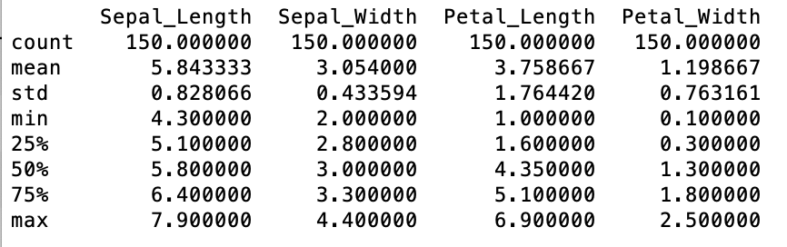
print(iris.describe())

The code output shows that there are no null values, the RangeIndex has 150 entries from 0 to 149. The four measurement columns each consist of 150 non-null float64 numbers.

The three classes or species types of iris in the data set are Iris-setosa, Iris-versicolor and Iris-virginica

Here are some summary statistics for the iris DataFrame:

The initial exploration of the Iris DataFrame shows that there are 150 rows and 5 columns of data. Each row corresponds to an individual observation of an iris plant.
The columns show the individual measurements (in centimetres) of the length of the sepal, the length of the petal, the width of the sepal and the width of the petal.
The mean of the Sepal length is greater than the mean of the other three measurements.
The measurements of the petal width has the lowest average measurements.
The standard deviation in the petal lengths shows the highest variability of the four measurements at 1.76 while the standard deviations of the petal width is approx 0.43.
The shortest petal in the data set is 1 cm while the longest petal is 6.9 cm.
The widths of the petals vary from 0.1 cm to 2.5 cm.
The shortest sepal in the data set is 4.3 cm while the longest sepal is 7.9 cm.
The narrowest sepal is 2cm while the widest sepal is 4.4 centimetres.
There are 50 observations in each class.

Visualising the Iris data set

A picture tells a thousand words. Visualising the data was key to Edgar Anderson’s reaching his conclusions, although he did not have the convenience of a programming language such as python to do so!. Fisher also visualised the iris dataset using histograms.

I will now look at some visual summaries of the Iris data set using some plots and see what it shows. Using python to do so is som much easier than the work that Anderson did by hand.

Plots can show how variables in the Iris data set relate to each other and trends and patterns that may indicate relationships between the variables.
In particular I am looking to see at how linearly separable the three different classes of Iris appear as this seems to be a key reason for the Iris data set being so widely used the machine learning.

The matplotlib - pyplot package can be used to create a graph or plot of the Iris Data set. The pandas library also has some built in methods to create visualisations from DataFrame and Series objects which are based on the matplotlib library.

A histogram is a representation of the distribution of data. It charts the data using adjacent rectangular bars and displays either the frequency or relative frequency of the measurements on the interval or ratio scale. The pandas hist function calls matplotlib.pyplot.hist on each numerical series in the DataFrame, resulting in one histogram per column.

The histograms here show the distribution of each of the the measurements attributes across the iris data set.

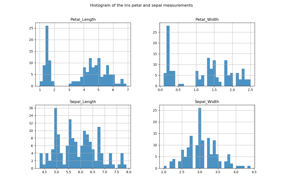
The histogram for the petal lengths show a clear group of observations having petal lengths that are much smaller than the rest of the observations and similarly so with the petal widths. The sepal lengths show quite a bit of variation with a number of peaks while sepal widths seem to be centred around 3 cms but with a few smaller peaks at both sides of 3 cms.

A boxplot is a very useful plot as it shows various statistics in one go, including the median, quantiles, interquartile range, outliers etc. The length of the box is the interquartile range and measures the variability in the data set. The interquartile range (IQR) is the middle 50% of the data and can show the spread or variation of the data. The whiskers show if the data is skewed in one direction or the other. The median is the line through the box.

Along with showing the distribution of values within each category, boxplots also allow for comparisons across the various classes. The boxplots below are generated using the seaborn library. The seaborn library demonstrates some of its plotting functions for visualising dataset structure using the Iris dataset which is built into the library.

In the boxplot below, the columns containing the categorical variable Class and the petal and sepal length measurement variables are passed in as the x and y parameters to the boxplot. Four plots are being plotted on a 2 by 2 grid. I am also specifying that the y axis should not be shared between plots and setting the figure size. The appearance of the plot can be changed by setting the figure aesthetics including the theme and the colour palette. The hue is set to ‘Class’ so that the points will be coloured on the plot according to their Class/species type.

sns.set(style="ticks", palette="pastel")
f, axes = plt.subplots(2, 2, sharey=False, figsize=(12, 8))
f, axes = plt.subplots(2, 2, sharey=False, figsize=(12, 8))
sns.boxplot(x="Class", y="Petal_Length",data=iris, ax = axes[0,0])
sns.boxplot(x="Class", y="Sepal_Length", data=iris, ax=axes[0,1])
sns.boxplot(x="Class", y="Petal_Width",hue = "Class",data=iris, ax=axes[1,0])
sns.boxplot(x="Class", y="Sepal_Width", data=iris, ax=axes[1,1])
# adding a title to the plot
f.suptitle("Boxplot of the Petal and Sepal measurements by Iris plant Species")
plt.show()

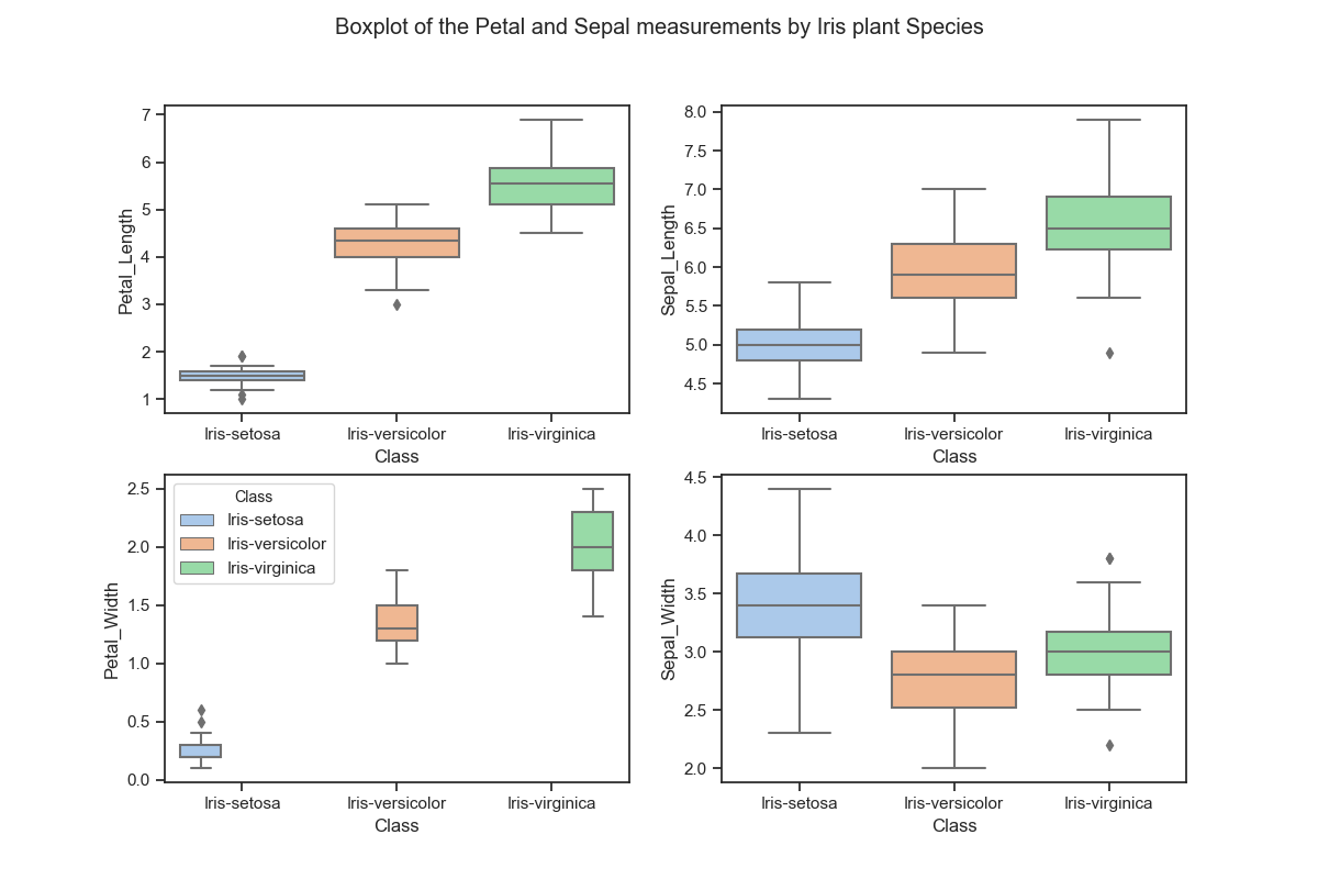
The boxplot proves to be a very useful plot for clearly showing the differences in the distributions of the measurements across the three iris species in the dataset. The Iris Setosa stands out from the other two classes as having much smaller petals. There does not appear to be many outliers.

The Iris data set can be separated into three subset groups based on their known class or species of Iris plant.

There are several ways of selecting data from the DataFrame which is detailed on the Indexing and selecting data section of the the pandas documentation.

Columns can be selected by name using square brackets. For example, iris["Sepal_Length"] will return the column ‘Sepal_Length’ of the iris DataFrame. A column of data can also be retrieved from the Iris DataFrame using dict-like notation or by attribute such as iris.Petal_Width. Index operators can be used to select a subset or rows and columns using the loc attribute for axis labels or iloc attribute for integers. An index into the dataframe can used to retrieve one or more columns, either with a single value or a sequence of values for the index.
Boolean Indexing can be used to select rows from the Iris DataFrame by filtering the data for rows that correspond to a a particular class or species of the iris plant, for example:

# select from the iris DataFrame only the rows where the Class equals the string "Iris-setosa"
iris_setosa = iris[iris['Class'] == "Iris-setosa"]

# subsetting to meet criteria using `isin` operator and boolean masks. Select columns where class is iris-versicolor or Iris-virginica
values =  {'Class': ['Iris-versicolor', 'Iris-virginica']}
row_mask = iris.isin(values).any(1)
iris[row_mask].head()

Subsets of the Iris data for each Class of Iris plant can be obtained by using one of these methods above. Another way is by using the pandas groupby function and this is the method I use in the script to split the Iris data set into subset groups by their class/species of Iris plant.
groupby allows the data to be easily sliced and diced and then to look at the characteristics and statistics of each subset group or to apply functions to each group.

The groupby function can be used to group the data by a Series of columns. A groupby operation involves three steps. First splitting the data into groups of observations based on some criteria, secondly applying a function to each group independently and thirdly the results are combined into a result object.

Here is the code I use in the script to calculate group statistics for each species or class of iris plant in the dataset. I wrapped the functions in print statements to make it easier to understand the output of the code when the full python script is run.

print("using groupby to split the iris dataframe by Class of iris species")
iris_grouped = iris.groupby("Class")
iris.groupby("Class").count()
print("The number of observations for each variable for each Iris species in the data set are as follows: \n \n",iris.groupby("Class").count())
print("The mean or average measurement for each group of Iris Species in the dataset is \n",iris.groupby('Class').mean())
print("the first observation in each Class of Iris plant in the Iris dataset are: \n  \n",iris.groupby("Class").first())
print("the last observation in each Class of Iris plant in the Iris dataset are: \n  \n",iris.groupby("Class").last())
print("The first three rows for each Class of Iris plant in the Iris dataset are: \n\n",iris.groupby("Class").head(3))
print("The last three rows for each Class of Iris plant in the Iris dataset are: \n\n",iris.groupby("Class").tail(3))
print("The maximum value for each measurement for each Class of Iris plant in the Iris dataset are: \n\n",iris.groupby("Class").max())
iris.groupby("Class").min()print("The minimum value for each measurement for each Class of Iris plant in the Iris dataset are: \n\n",iris.groupby("Class").min())

Summary statistics for each Class of iris plant in the dataset can be obtained using the describe method on the GroupByobject.
(The results can be transposed to make them easier to read.)

print(iris.groupby("Class").describe())

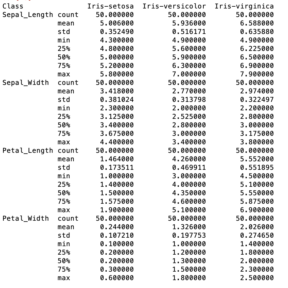
The statistics at the Iris species or class level show that the average petal length for an Iris Setosa is much smaller at 1.464 cm than the other two classes. The average petal length for the Versicolor is 4.26 while the Iris Virginica has the largest average petal length of 5.552 centimetres which is almost four times greater than the petal length of the Iris Setosa. The petal measurements of the Iris Setosa is much less variable than that of the other two species.

The average petal width of the Setosa is also much smaller than the average petal widths of the other two species. In fact the petal width of the Setosa is about twelve times smaller than the petal width of the Virginica. There is less variability in petal widths in all three species though compared to the variability in the petal length. There is not such a large difference between the sepal lengths of the three Iris species, although the Setosa is again showing the smallest average measurements. The average sepal width of the Setosa however is actually larger than the averages for the other two species. The average sepal width for the Setosa is 3.42 centimetres compared to an average of 2.77 cm for the Versicolor and 2.97 for the virginica. This is also shown in the minimum and maximum measurements for the three species.

From the summary statistics of the sepal and petal measurements by class type it would seem that the differences between the Iris Setosa and the other two species is more pronounced that any other differences between the three classes.

Scatterplots of the Iris data set.

A scatter plot is a useful plot as it visually shows how the different variables or features in the data set correlate with one another. It is a graph of the ordered pairs of two variables. One variable is plotted on the x-axis while the other variable is plotted on the y-axis. A scatter plot can be used to visualize relationships between numerical variables such as the petal measurements and the sepal measurements in the Iris data set.
The Iris data set is a multi-class data set as there are three classes to which the observations could belong to. The seaborn library has a pairwise scatter plots function that is suitable for dealing with this. The pairplot() function shows all pairwise relationships and the marginal distributions that can be conditioned on a categorical variable. pairplot creates a grid of axes with each variable in the data is shared in the y-axis across a single row and in the x-axis across a single column. The diagonals show plots of the univariate distribution of the data for the variable in that column.

sns.pairplot(iris, hue="Class")

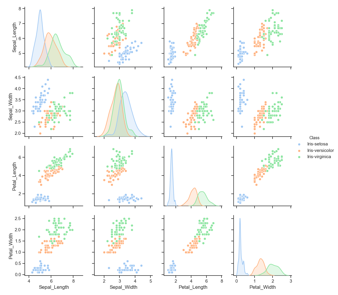
A linearly separable data set is one where the observations or data points can be separated by a straight line drawn through the data.

The scatter plots in the pairwise grid of plots shows how the Iris Setosa is clearly different from the other two species. However they also show that it is not so simple a matter to separate the other two classes from each other as there is a bit of overlap in the data points.

Correlation is a statistical method used to determine whether a linear relationship between variables exists and shows if one variable tends to occur with large or small values of another variable.
The correlation statistics are computed from pairs of arguments. The correlation of the measurements can be got using the corr method on the Iris DataFrame. If there is a strong positive relationship between the variables, the value of the correlation coefficient will be close to 1, while a strong negative relationship will have a correlation coefficient close to -1. A value close to zero would indicate that there is no relationship between the variables.

The correlation coefficients between measurement variables:

iris.groupby("Class").corr()

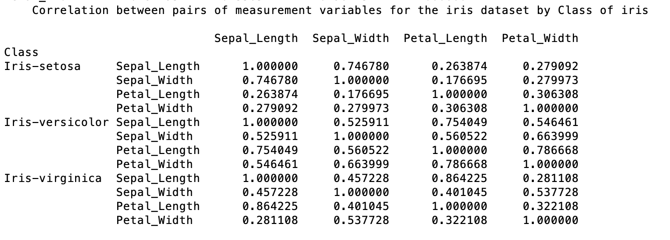
The correlation matrix shows the following relationships between the measurement variables:

a high correlation between sepal length and sepal width for the Iris Setosa at almost 0.75 while the correlation between the sepal measurements is nearer to 0.5 for both the Iris Versicolor and almost the Iris Virginica.
a strong positive correlation between the petal length and petal widths for the Iris Versicolor only
a very strong relationship between the petal length and the sepal length for the Iris Virginica at over 0.86
The Iris Versicolor also shows a strong correlation between the petal length and the sepal length at 0.75