California Housing Prices
By Angela C
October 5, 2021
Reading time: 8 minutes.
I am reading Hands on Machine Learning with Scikit-learn, Keras and TensorFlow by Aurélion Géron and will make a few notes here for reference.
Chapter 2 works through an example project from end to end using the California Housing dataset from the StatLib repository. The dataset is based on data from the 1990 California census from the StatLib repository and includes metrics such as population, median income and median house price for each block group in California. (A block group is the smallest geographical unit for which the census publishes data, typically containing 600 to 3,000 people.)
The main steps in a machine learning project that are outlined in this chapter include looking at the big picture, getting the data, discovering and visualising the data to gain insights, selecting and training a model, fine-tuning the model, presenting your solution and then launching, monitoring and maintaining the system.
The task is to use California census data to build a model of housing prices in California. The model should learn from the data and be able to predict the median house prices in any Californian districts given a number of features from the dataset.
It is a supervised learning task as it involves labeled training instances which have the expected output, a multiple regression task as the aim is to predict values using multiple features and a univariate regression problem as there is only a single value to be produced for each district. A multivariate prediction task would aim to predict multiple values per district.
The dataset is small enough to fit in memory and is self-contained and therefore suitable for batch learning. For very large data, an online learning technique could be used or the batch learning could be split across multiple servers using MapReduce.
The dataset is also available from the sklearn-datasets module.
All attributes in the dataset except one are numerical.
This dataset has some null values for the total_bedrooms attribute. These were purposely removed from the original dataset by the author to have some missing values in the dataset to work with. An additional categorical attribute ‘ocean_proximity’ was also added to this dataset by the author to discuss dealing with categorical data.
Selecting Performance Measures
-
The Root Mean Square Error (RMSE) is a performance measure that is suitable for regression. The RMSE indicates how much error the system makes in its predictions. It gives a higher weight to large errors. The RMSE corresponds to the Euclidian norm also called the $l_2$ norm. $||.||_2$ or $||.||$.
-
The Mean Absolute Error (MAE) is another performance measurement (also known as average absolute deviation) and corresponds to the Manhattan Norm or $l_1$ norm.
Both the RMSE and MAE measure the distance between the vector of predictions and the vector of target values. The RMSE can be more sensitive to outliers than the MAE but when outliers are exponentially rare (a bell-shaped curve) then the RMSE performs well and is commonly used in regression tasks.
Some summary statistics and histograms to see the distribution of each variable.
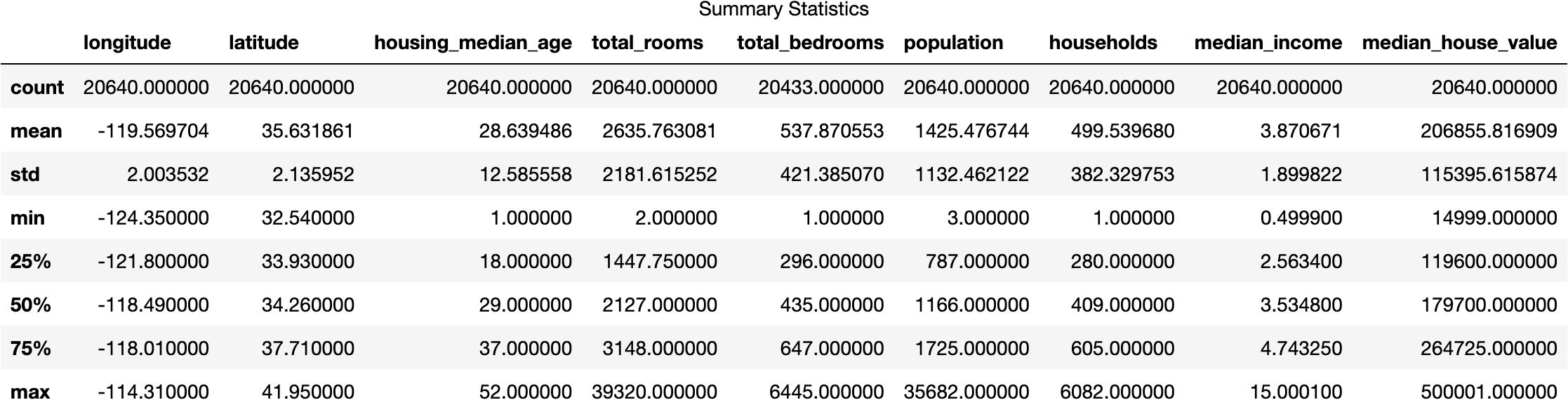
Summary Statistics of the California House Prices dataset
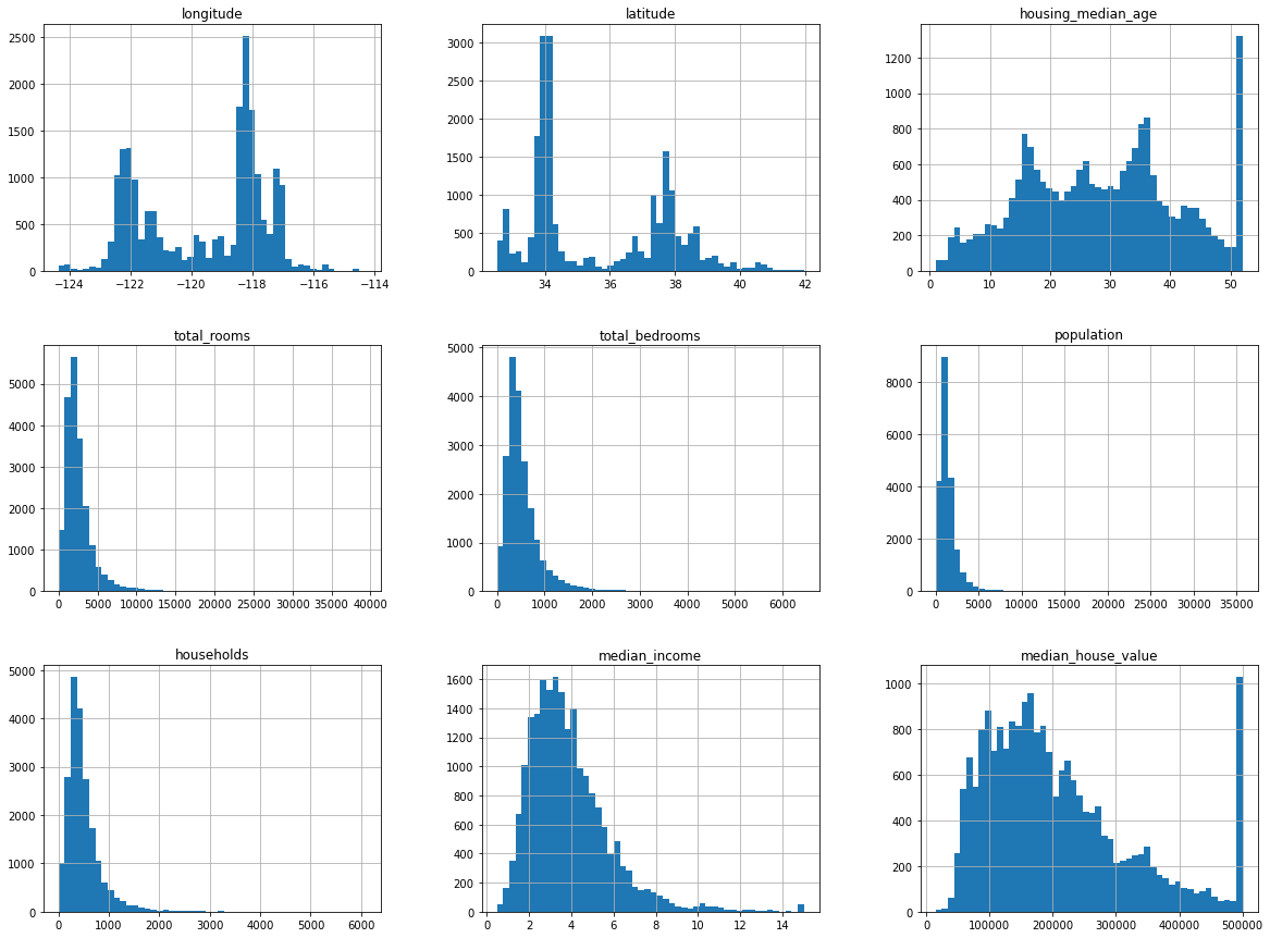
Histograms of the attributes in the dataset
Creating a Test Set
To prevent data snooping bias a test set should be created and set aside before going any further. Otherwise you could be tempted to select a particular model based on what you see and end up with an over-optimistic generalizaton error.
Scikit-learn has some functions for splitting datasets into multiple subsets in various ways such as the split_train_test() function. It takes a random_state paramater that allows you to set the random generator seed. It can also be passed multiple datasets with the same number of rows and it will split them on the same indices which is very useful when the labels are in another dataframe.
- Pure random sampling is fine when the dataset is large (relative to the number of attributes) but otherwise could result in a signficant sampling bias.
- Stratified sampling splits a population into strata (homogenous subgroups) called strata and selects the correct number of instances from each strata to guarantee that the test set is representative of the overall population.
- It is important to have enough instances for each stratum, otherwise the estimate of a stratum’s importance may be biased. There should not be too many strata and each stratum should be large enough.
Median income in the area is considered a very important attribute when predicting house prices in an area so the test set should be representative of the various categories of income in the entire datasets.
The median income variable is a continuous numerical variable but you can create from an income category attribute from this using pandas pd.cut. The new income categories can be used when doing stratified sampling using Scikit-learn’s StratifiedShuffleSplit class. The histogram of median income shows where most of the values are clustered.
- Compare the category proportions in the test set to the proportions in the full dataset.
from sklearn.model_selection import StratifiedShuffleSplit

split = StratifiedShuffleSplit(n_splits=1, test_size=0.2, random_state=42)
for train_index, test_index in split.split(data, data["income_cat"]):
    strat_train_set = data.loc[train_index]
    strat_test_set = data.loc[test_index]
Comparing the income proportion in the full dataset to the test set generated with stratified sampling to the test set generated with purely random sampling, the results showed that the test set using stratified sampling has income proportions much closer to the actual proportions in the full dataset while the test set created using purely random sampling is skewed.
(The new income category can be removed from the dataset.)
Visualising the data to gain insights
The next step is to visualise the data to gain insights. This should be performed on the training set only. The test set should be set aside.
If the training set is very large, you can use an exploration sampled from the (training) set. A copy can be made (using pd.cut) of the training set to avoid damaging it.
The data contains geographical location data which can be used to make a scatter plot of all the districts. Setting alpha values to deal with high density of points on the map.
The visualisation show that housing prices are very much related to location (close to ocean) and to population density. However some of the Northern Californian coastal districts do have lower median values and some inland areas have higher median values than other inland areas. Therefore being close to the ocean is not a simple rule.
A clustering algorithm could be added to detect the main cluster and add new features measuring the proximity to the cluster centres.
Correlations:
The standard correlation coefficient also known as Pearson’s R can be calculated between every pair of attributes using using corr() method.
The pandas scatter_matrix() function plots every numerical attribute against every other numerical attribute with a histogram of each attribute along the diagonal.
It is important to note that correlations coefficients only measure linear correlations and may miss out on non-linear relationships.
Looking at how each attribute correlates with the median house value:
Median house prices tend to go up when median incomes go up but they tend to go down when you go north as the slight negative correlation with latitude shows. There is a very strong correlation between median income and median house values with an upwards trend and the points are not too dispersed.
The horizontal line at 500,000 shows the price cap in the dataset while there are other horizontal lines also visible around 350k and 450k. Géron notes that you should consider removing the corresponding districts to prevent your algorithm from learning to reproduce these data points.
Trying out some attribute combinations
These are several ways to explore the dataset and gain some insights. If there are any quirks in the data these should be identified and possibly cleaned up before feeding the data into a machine learning algorithm.
The histograms aboved showed that some attributes have tail heavy distributions which may need to be transformed (perhaps by calculating the logarithm).
Various attribute could also be combined together to create new attributes. An example would be creating a rooms per household attribute by calculating ‘total_rooms’ as a proportion of the ‘households’ attribute. The total number of rooms in a district is not very useful without knowing know how many households there are. Bigger houses with more rooms tend to be more expensive.
Another attribute could be created in a similar way from the ‘total_bedrooms’ and ‘total_rooms’ attributes to show the number of bedrooms to the total_rooms. The population per household could be calculated from the ‘population’ and ‘households’ attributes.
Having done so, the new rooms_per_household attributes is more correlated with median house value than the total number of rooms or total number of bedrooms. The bigger the house, the more expensive the house.
The bedrooms_per_room attribute is more correlated (but negatively) with median house values that total number of bedrooms. Houses with a lower bedroom / room ratio tend to be more expensive.
corr_matrix = housing.corr()
corr_matrix["median_house_value"].sort_values(ascending=False)
median_house_value          1.000000
median_income               0.687160
rooms_per_household         0.146285
total_rooms                 0.135097
housing_median_age          0.114110
households                  0.064506
total_bedrooms              0.047689
population_per_household   -0.021985
population                 -0.026920
longitude                  -0.047432
latitude                   -0.142724
bedrooms_per_room          -0.259984
Name: median_house_value, dtype: float64
The next step is prepare the data for Machine Learning algorithms.
-
Géron, Aurélien. Hands-On Machine Learning with Scikit-Learn, Keras, and TensorFlow O’Reilly Media
-
Launch, model and maintain This section of the chapter outlines how a trained model can be deployed to a production environment.